※ In this post, vectors are represented using “row vectors” as the default direction. For more detailed explanation of this, please refer to the first section “Data representation using row vectors”.
Prerequisites
To better understand this post, it is recommended that you be familiar with the following content:
If you need a more detailed explanation of the covariance matrix, please refer to the following post:
Data representation using row vectors
In mathematics, it is more common to view column vectors as the default direction when representing vectors. In other words, a vector $x$ of arbitrary dimension $n$ is usually represented as follows.
\[\vec{x}=\begin{bmatrix}x_1 \\ x_2 \\ \vdots \\x_n\end{bmatrix} % Equation (1)\]
In this case, the matrix must go to the left of the vector. The product of an arbitrary $n\times n$ dimensional matrix $A$ and an $n$ dimensional column vector $x$ is represented as follows.
\[Ax % Equation (2)\]
Furthermore, the dot product between column vectors can be expressed using the transpose operator as follows. For any $n$-dimensional vectors $\vec{x}$ and $\vec{y}$,
\[dot(\vec x, \vec y)=\vec x^T\vec y % Equation (3)\]
However, in data science, for some reason unknown, a single data point is usually treated as a row vector and used. In other words, an arbitrary $d$-dimensional vector $x$ is represented as follows.
\[\vec{x}=\begin{bmatrix}x_1 & x_2 & \cdots & x_d\end{bmatrix}% Equation (4)\]
In this case, the matrix must go to the right of the vector. The product of an arbitrary $d\times d$ dimensional matrix $R$ and an $d$-dimensional row vector $x$ can be written as follows.
\[x R % Equation (5)\]
Furthermore, the dot product between row vectors also uses the transpose operation, but the transposed vector is on the right. In other words, for any $d$-dimensional row vectors $\vec{x}$ and $\vec{y}$,
\[dot(\vec x, \vec y)=\vec x \vec y^T % Equation (6)\]
Going further, in data science, it is common to have a data set $\mathcal D$ with $n$ samples and $d$ features represented as an $n\times d$ dimensional matrix. In other words, if more sample data is added, one row is added. In other words, each data point is treated as a “row vector.”
In this post, the default direction of vectors is set to “row vectors.”
Contextual relative distance
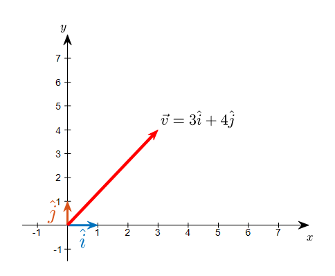
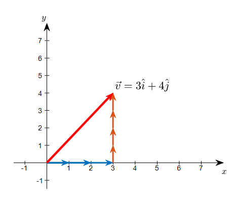
Consider two vectors $\vec x$ and $\vec y$ as shown below.
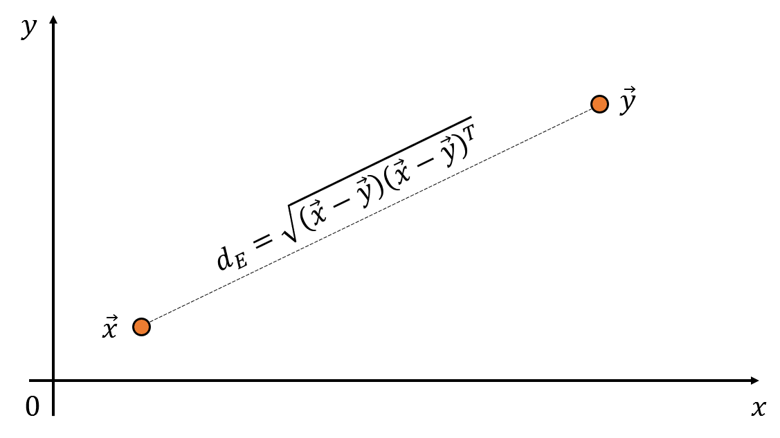
Figure 1. The distance between two vectors in space can be calculated using the dot product of the vectors.
What formula should be used to calculate the Euclidean distance between an arbitrary point $\vec x$ and $\vec y$? The distance can be calculated using the difference and dot product of the two vectors. This distance is called the Euclidean distance.
\[d_E = \sqrt{(\vec x-\vec y)(\vec x-\vec y)^T} % Equation (7)\]
However, if we consider other data points in the vicinity, we may need to reconsider whether to use an absolute distance between two points.
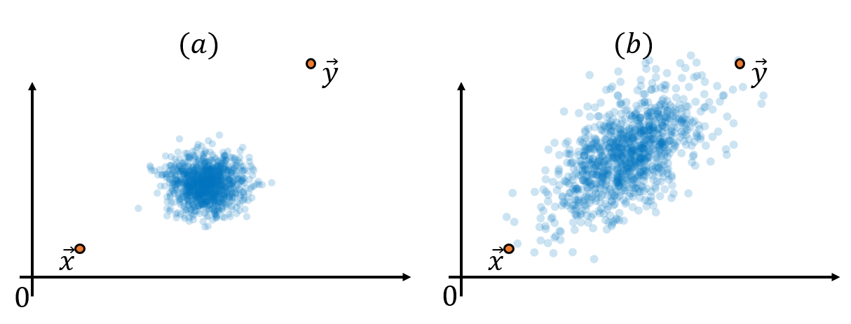
Figure 2. The distance between two points, taking into account the context of other data points, may need to be calculated differently.
In the above figure, (a) can be seen as points that are quite away from the distribution of blue data, while (b) is in a relatively less deviated location from the distribution. In other words, considering the “context” of other data points, the distance between the two vectors in Figure 2 (a) may be farther than the distance between the two vectors in Figure 2 (b).
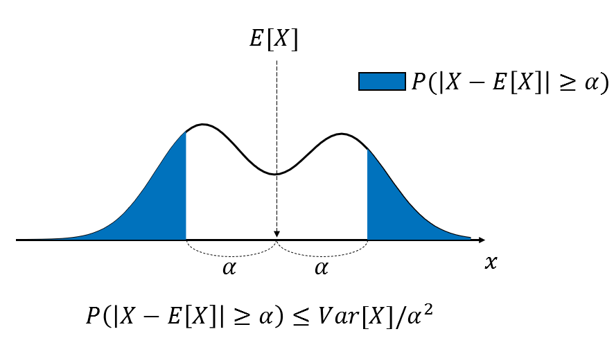
The ambiguous expression “context” can be expressed more mathematically as “standard deviation.” If we can assume that the data is in the form of a normal distribution, we can use the properties of the standard deviation of a normal distribution to see that there is 68, 95, and 99.7% of the data coming in at a distance of 1, 2, and 3 standard deviations away from the mean (center).

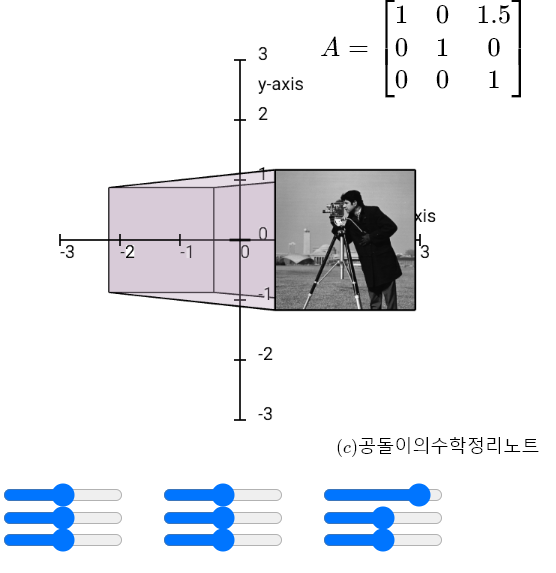
Figure 3. How much data is included when moving 1, 2, and 3 standard deviations away from the center in a normal distribution? (68–95–99.7 rule)
In other words, standard deviation contours can be displayed based on the standard deviation, as in the figure below. And these contours become indicators of “contextual” distance.
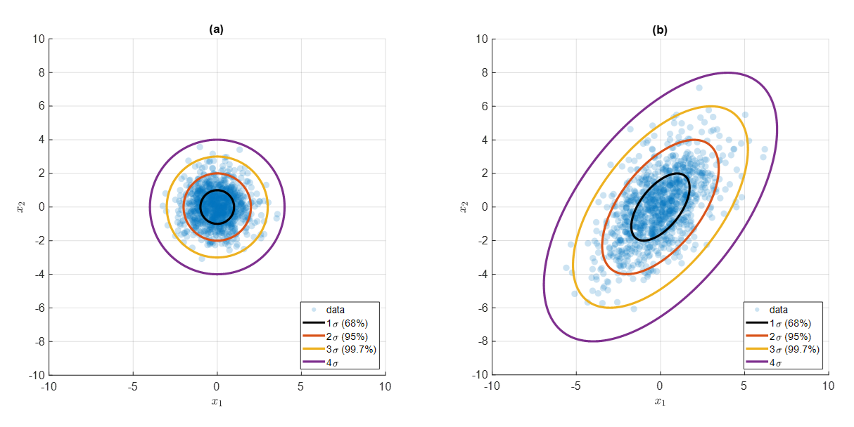
Figure 4. A contour that represents the distance from the mean in standard deviation units of 68, 95, and 99.7%
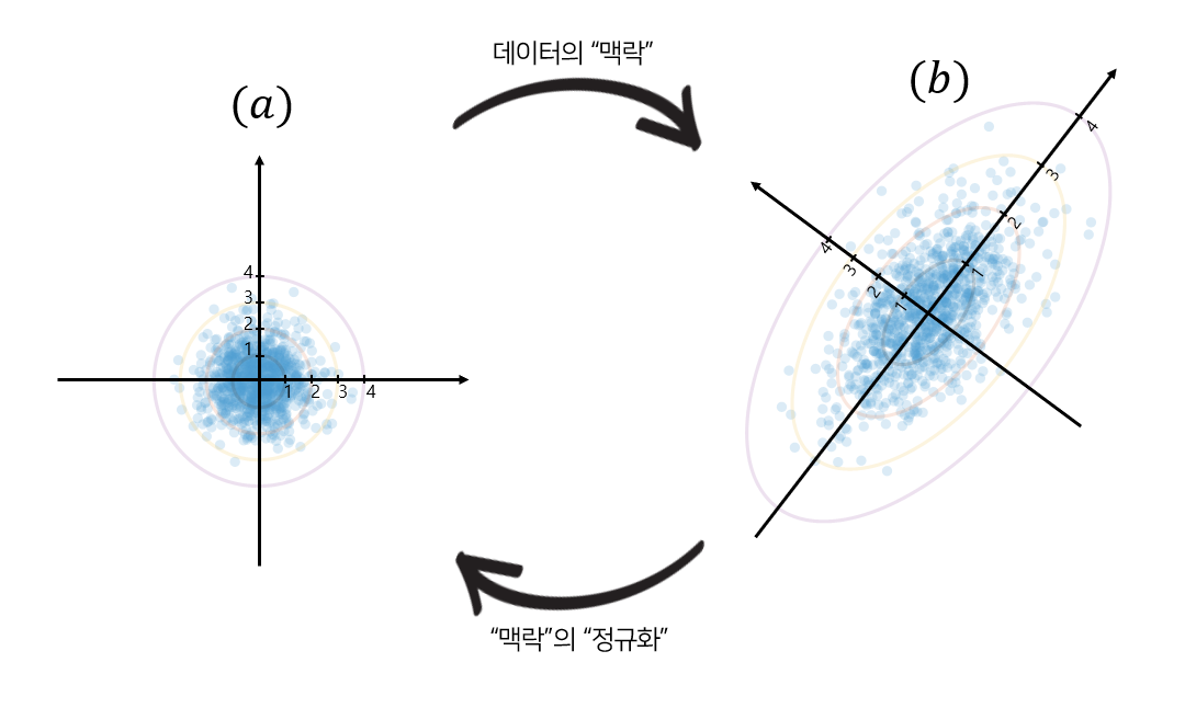
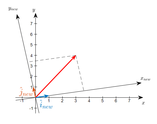
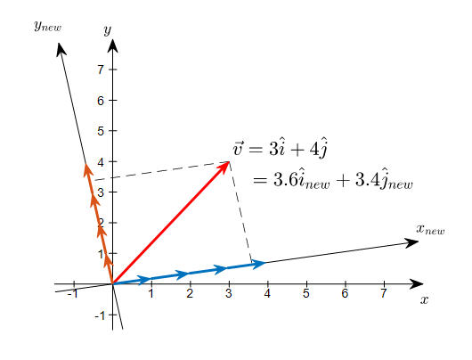
And by reducing the ellipsoidal shape in (b) of figure 4 to a unit circle as in (a) of figure 4, we can normalize the standard deviation that represents the “context” of the data. Let’s take a look at the transformation of the vector space using new axes corresponding to standard deviations 1, 2, 3, etc. as shown in figure 5 below.
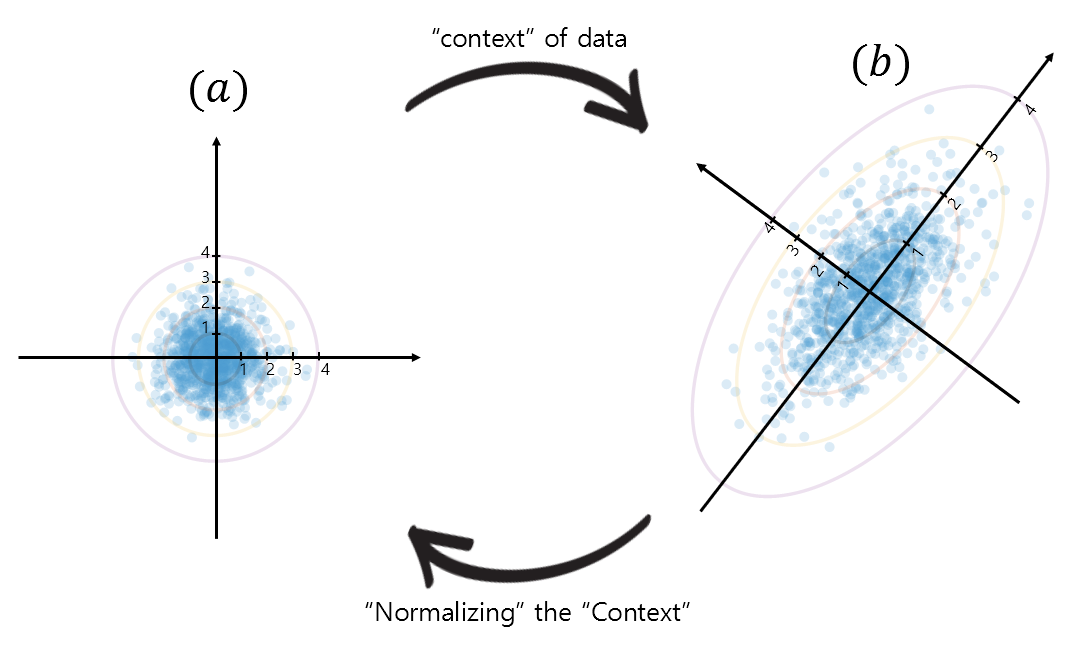
Figure 5. Representation of the "context" of the data and transformation of the data (vector) space to "normalize" the "context"
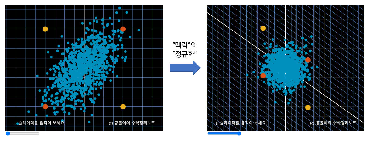
This process is performed in the applet at the top of this post. Let’s look at the left of Figure 6. When considering the “context” of the given data, we should judge that the yellow points are farther away than the orange points. This is a complicated task as the Euclidean distance must be calculated while considering the “context”. However, if we normalize the “context” as in the right of Figure 6, the distance between the yellow points is already considered as farther away by simply calculating the Euclidean distance. This is because the original data (vector) space was transformed while taking into account the “context” of the given data in the process of “normalizing” the “context”.
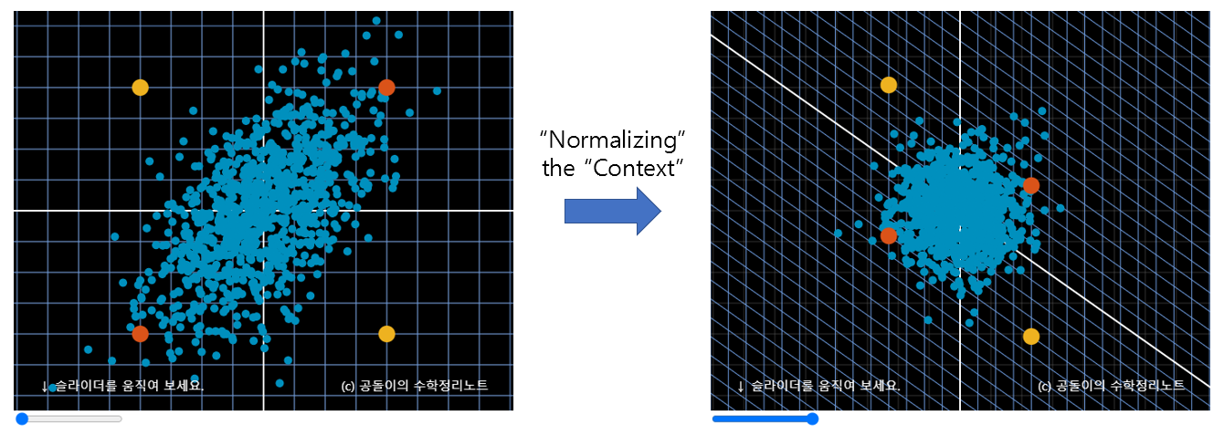
Figure 6. The Euclidean distance measured after "normalizing" the "context" already becomes a distance that takes into account the "context".
Investigating the “context” through the distribution of the given data and normalizing it before calculating the Euclidean distance is the Mahalanobis distance.
\[d_M = \sqrt{(\vec x-\vec y)\Sigma^{-1}(\vec x-\vec y)^T} % Equation (8)\]
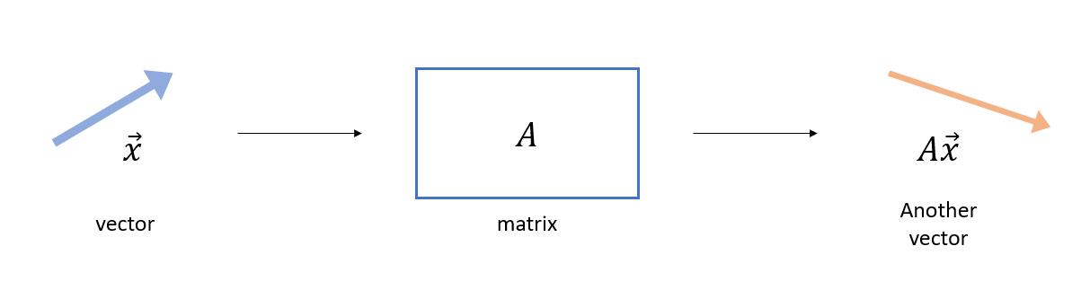
The transformation of the vector space can be represented by a matrix. Specifically, the matrix that represents the “context” of the data is related to the covariance matrix, and the matrix that rotates it back is related to the inverse matrix of the covariance matrix. From now on, let’s try to understand how to grasp the “context” of the data mathematically. Also, let’s examine how to perform “normalization” of the “context” in more detail.
The Meaning of the Covariance Matrix and its Inverse Matrix
Basic Understanding of iid Gaussian Distribution Samples
Before understanding the structure of the data, we first need to understand the properties of iid (independent and identically distributed) normal distribution samples. Although the terminology may seem difficult, there is nothing difficult once we look at it carefully. iid is one of the simplest methodologies for extracting random data samples.
To explain iid, let’s break it down into the following assumptions:
- The extracted data is independently extracted.
- The extracted data is extracted from the same probability distribution.
Furthermore, assuming that the probability distribution extracted here is a normal distribution, the extracted samples can be expressed as “independent and identically distributed normal random variables.”
This time, let’s stack multiple iid normal random variables $z_1, \cdots, z_d$ side by side as $Z\in\mathbb{R}^{n\times d}$. In particular, for convenience of calculation, assume a standard normal distribution.
\[Z =\begin{bmatrix} | & | & & |\\ z_1 & z_2 & \cdots & z_d\\ | & | & & |\end{bmatrix} % Equation (9)\]
\[\text{where } z_1, z_2, \cdots, z_d \text{ are i.i.d. normal random variables with mean 0 and variance 1}\notag\]
As we have extracted samples from a standard normal distribution, we can confirm the following. Since the mean of the extracted distribution is 0,
\[\mathbb{E}[z_i]=0 \text{ for } i = 1, 2, \cdots, d % Equation (10)\]
Moreover, let’s also consider the following given that the variance of the extracted distribution is 1.
\[\mathbb{E}\left[Z^TZ\right]
= \mathbb{E}\left [\begin{bmatrix}
z_1^T z_1 & z_1^T z_2 & \cdots & z_1^Tz_d \\
z_2^T z_1 & z_2^T z_2 & \cdots & z_2^T z_d \\
\vdots & \vdots & \ddots & \vdots \\
z_d^T z_1 & z_d^T z_2 & \cdots & z_d^Tz_d
\end{bmatrix}\right ] % 식 (11)\]
Here, for $i=1,2,\cdots, d$, $\mathbb{E}\left[z_i^T z_i\right]$ is equal to the sum of $n$ variances of 1, so $\mathbb{E}\left[z_i^T z_i\right]=n$. Furthermore, since $z_i$ is extracted independently, for different $i$ and $j$, $\mathbb E \left[z_i^T z_j \right]=0$.
Therefore, equation (11) can be represented as
\[\text{Equation (11)} \Rightarrow \begin{bmatrix}
n & 0 & \cdots & 0 \\
0 & n & \cdots & 0 \\
\vdots & \vdots & \ddots & \vdots \\
0 & 0 & \cdots & n
\end{bmatrix} = n I\]
Here, $I$ is a unit matrix of dimensions $d \times d$.
Another way to understand the given data
Suppose that 1,000 aliens living on Mars were randomly selected and their height and weight were measured. Amazingly, the average height was 10cm and the average weight was 8kg. Suppose that the data is arranged in a table, which roughly looks like the following.
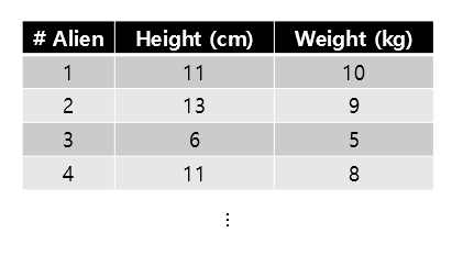
Figure 8. Table summarizing the height and weight of aliens on Mars (rounding up to the 4th alien)
The height and weight data of 1,000 aliens can be found here.
Let’s call the data that arranges the height and weight $\mathcal D$. Also, if the number of aliens sampled is denoted as $n$, and the number of features such as height and weight is represented as $d$, then $\mathcal D$ can also be viewed as the following matrix.
\[\mathcal D\in\mathbb{R}^{n\times d}\]
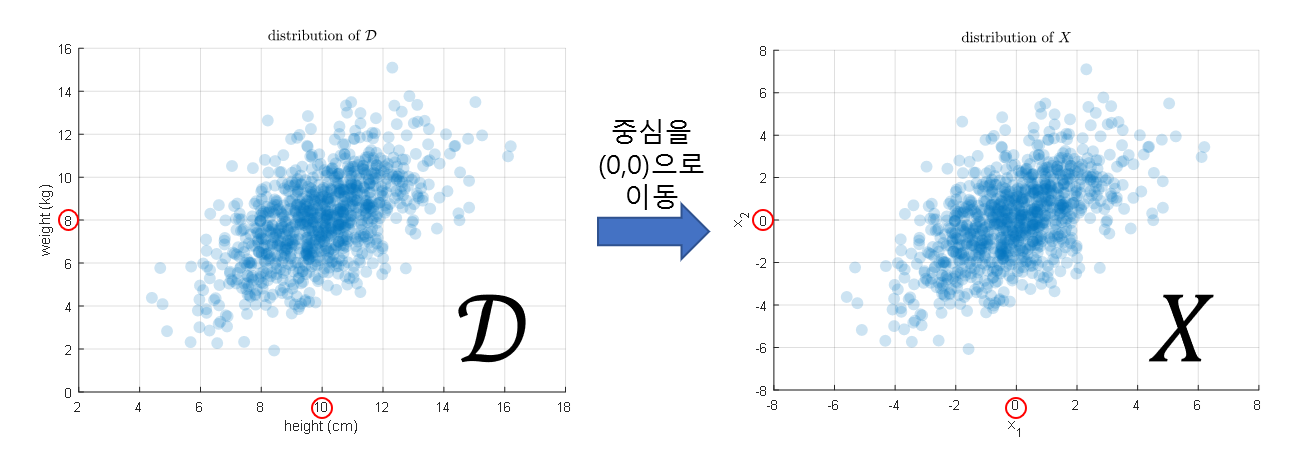
Although the data used this time was the height and weight of random 1000 aliens, it is possible to examine the distribution of any data. In order to understand the data distribution from a “new” perspective, let’s move all feature-wise mean values of the dataset to zero. Then, let’s view the new data, for which feature-wise mean values are zero, as data $X$.
If we plot the distributions of $\mathcal D$ and $X$, it is shown as below.
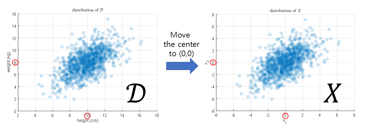
Figure 9. Distribution of height and weight data of aliens on Mars
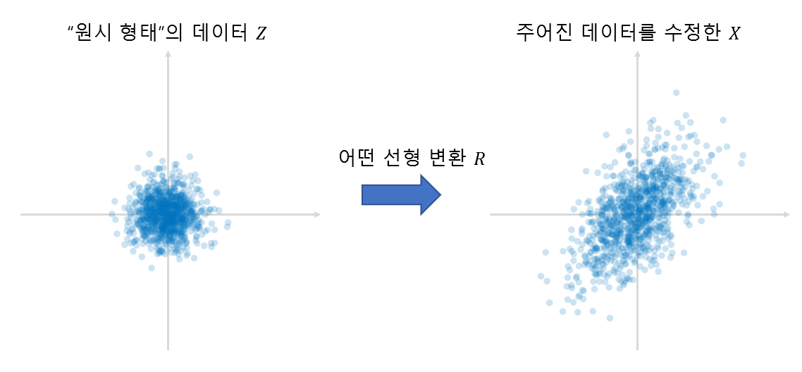
Now let’s try to understand the data $X$ as a result of linear transformation of raw data $Z$. Here, the reason why the linear transformation matrix $R$ is attached to the right of $Z$ is because we can see the basic direction of the vector as a row vector, as shown in equation (5).
\[X = ZR % Equation (14)\]
\[\text{where }Z \in \mathbb{R}^{n\times d} \text{ and } R \in \mathbb{R}^{d\times d}\notag\]
Let’s assume that all columns of $Z$ are datasets extracted from the standard normal distribution of iid (independent and identically distributed).
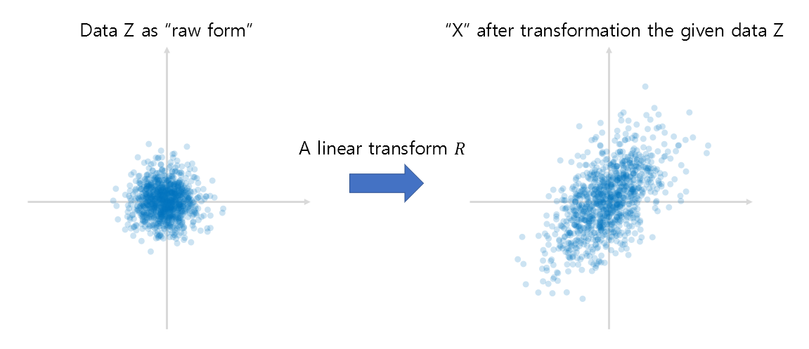
Figure 10. Understand the given data as $X$ modified from raw data $Z$ linear transformed.
From now on, let’s investigate the similarity between features. By investigating the similarity between features, we can understand the “context” or structural form of the data. That’s because, for example, if feature 1 and feature 2 are very similar, it means that they are highly correlated with each other. To do this, let’s calculate $X^TX$. $X^TX$ will have dimensions of $d \times d$, and it represents the inner product between features. If we calculate $XX^T$, we can expect that this will indicate the similarity between the data. Let’s see the process of calculating $X^TX$ in the figure below.
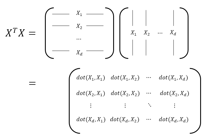
Figure 11. The process of calculating how similar each data feature is in order to compute the covariance matrix.
Here, using Equation (14) again, we have:
\[X^TX = (ZR)^TZR = R^TZ^TZR = R^T(Z^TZ)R % Equation (15)\]
Here, according to Equation (12),
\[X^TX \approx R^T(nI)R = nR^TR % Equation (16)\]
is established. Here, we used “$\approx$” because in actual data, the exact value of the expected value may not come out. And we can confirm the following fact:
\[R^TR \approx \frac{1}{n}X^TX % Equation (17)\]
What does equation (17) mean in the end? Equation (17) is a way of obtaining the “context” of the data of $X$ or the structural form of the data. This is almost identical to $R^TR$ for the linear transformation $R$ to transform the raw form $Z$ into the given data $X$. And the matrix that expresses the structural form of the equation (17) is called the covariance matrix. Let’s use $\Sigma $ to represent the covariance matrix here.
\[\Sigma = \frac{1}{n}X^TX % 식 (18)\]
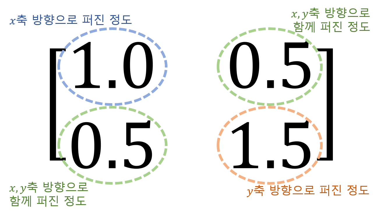
Note that there is also a way to divide by $n-1$ instead of $n$. The resulting covariance matrix obtained by dividing by $n-1$ instead of $n$ is called the sample covariance matrix. The covariance matrix is a useful way to describe the overall structure of the entire dataset and is especially closely related to multivariate normal distribution. If a dataset with two features follows a bivariate normal distribution, as in Figure 12, it can be said to follow one of the three major patterns below.
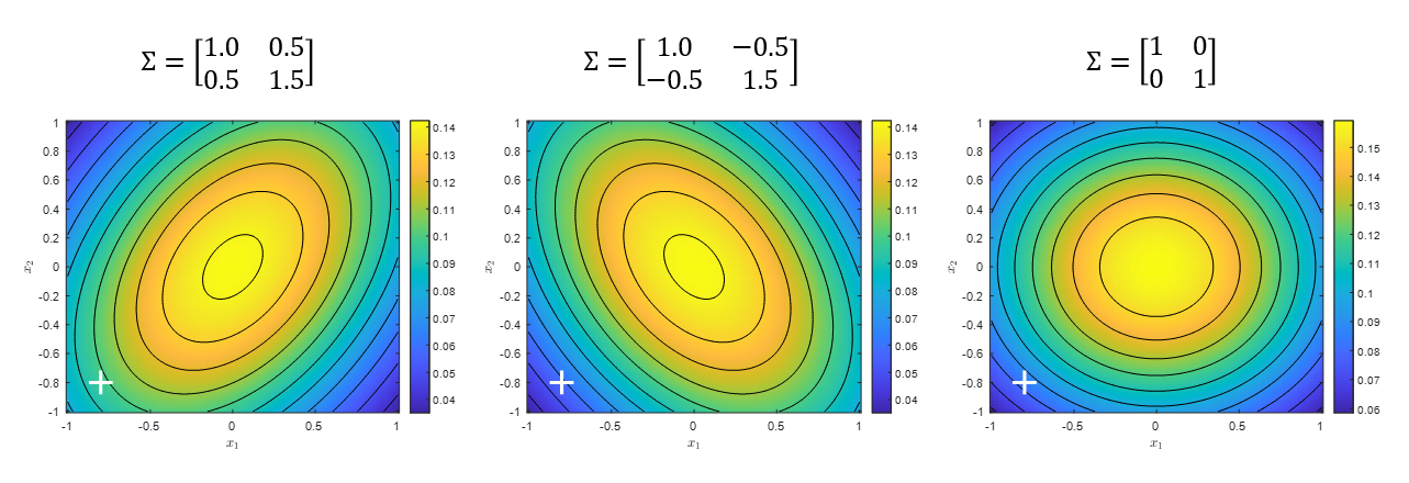
Figure 12. The three most representative forms of bivariate normal distributions.
Each element of the covariance matrix represents the variance or covariance of each feature. In other words, in the case of two features as in Figure 12, it represents how much data is scattered in the x-axis and y-axis for each feature, as well as how much variation is together between the first and second features.
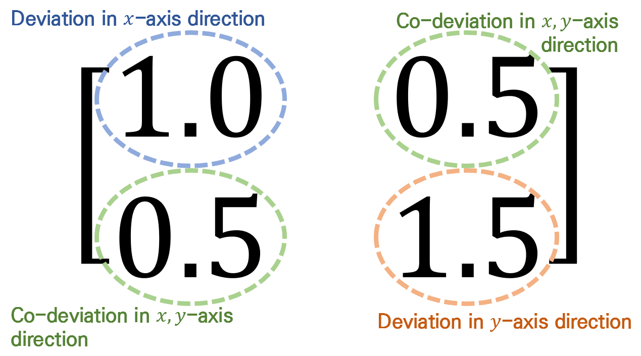
Figure 13. What each element of the covariance matrix represents.
Inverse matrix and normalization of context
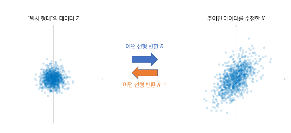
If the given arbitrary data is denoted as $x$ and its primitive form is denoted as $z$, then according to Equation (14), it can be seen that it is possible to restore the “context” of the given data to the form of primitive data by performing the following:
\[z=xR^{-1}\]
Here, the linear transformation using the inverse matrix is a method of restoring the vector space transformed by the given linear transformation $R$ to its original form. That is, if the process of changing from left to right in Figure 10 is the transformation performed by the original linear transformation $R$, the inverse transformation $R^{-1}$ can be seen as the transformation from right to left in Figure 10.
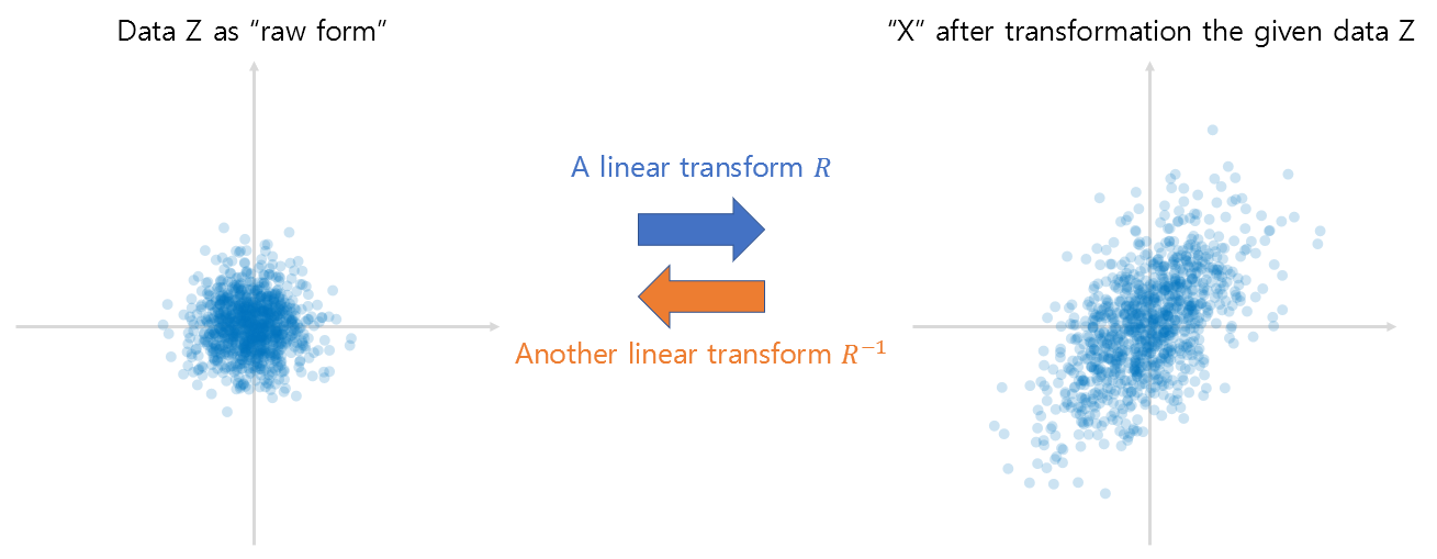
Figure 14. Linear transformation represented by matrix R and its inverse transformation.
Using Equation (7), we can calculate the distance $d_z$ between the origin and the primitive data vector space as follows:
\[d_z=\sqrt{zz^T}=\sqrt{(xR^{-1})(xR^{-1})^T}\]
\[=\sqrt{xR^{-1}(R^{-1})^Tx^T}=\sqrt{x(R^TR)^{-1}x^T}=\sqrt{x\Sigma^{-1}x^T}\]
Here, $\Sigma$ is the covariance matrix of the entire given dataset.
If we perform the same process as above for the distance between arbitrary vectors $x$ and $y$, we can modify the equation as follows, and this is the same as the Mahalanobis distance mentioned earlier:
\[\Rightarrow \sqrt{(x-y)\Sigma^{-1}(x-y)^T}\]
Contour lines and Principal Axes: Eigenvalues, Eigenvectors
※ The last chapter is somewhat advanced, and it is not necessary to understand it to understand the meaning of Mahalanobis.
※ To better understand the following content, it is recommended to understand the following:
Now let’s add the standard deviation and “contour lines” to understand the “context” of the data, as introduced in Figures 3 and 4. Talking about “contour lines” is one of the most important cores in understanding Mahalanobis distance.
First, let’s take another look at Figure 12. Figure 12 shows three representative forms of bivariate normal distributions that can be found. However, are these three shapes the only possible shapes for the distribution? Probably not. If we express the shape of the distribution with the two factors being how much it has rotated and how much it has been stretched, we can see that there will be countless shapes of the distribution. In other words, any distribution that can be represented by a multivariate normal distribution can be obtained by stretching and rotating a standard normal distribution.
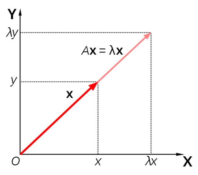
The method of expressing how much the given linear transformation has rotated and how much it has been stretched is called eigenvalue decomposition. The amount of rotation will indicate the direction of the new axis shown on the right in Figure 5, and the amount of stretching will indicate the length of one scale on the new axes. In addition, as discussed in the article on eigen decomposition, the rotation direction is represented by eigenvectors and the amount of stretching is represented by eigenvalues.
Let’s try to eigen-decompose the covariance matrix as follows:
\[\Sigma = Q\Lambda Q^{-1}=Q\Lambda Q^T\]
Here, since the covariance matrix is always a symmetric matrix, we can replace $Q^{-1}$ with $Q^T$.
Here, $Q$ and $\Lambda$ are matrices with eigenvectors and eigenvalues, respectively.
For example, if we eigen-decompose the covariance matrix of the first image in Figure 12, we can get the following result:
\[\begin{bmatrix}1 & 0.5\\0.5 & 1.5\end{bmatrix}=\begin{bmatrix}-0.8507 & 0.5257 \\ 0.5257 & 0.8507\end{bmatrix}\begin{bmatrix}0.6910 & 0 \\ 0 & 1.8090\end{bmatrix}\begin{bmatrix}-0.8507 & 0.5257 \\ 0.5257 & 0.8507\end{bmatrix}^T\]
And each column of $Q$ shows how much the standard normal distribution has been rotated, or more precisely, indicates the direction of the principal components (PCs). In addition, the diagonal elements of $\Lambda$ show how much the distribution has been stretched in each principal component direction. Refer to Figure 15 to understand this more visually.
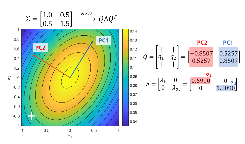
Figure 15. The eigenvalue decomposition of the covariance matrix allows us to represent how much the standard normal distribution has been stretched and rotated as a vector. Here, $\sigma_1$ and $\sigma_2$ represent how much PC1 and PC2 have been stretched, respectively.
To explain this result again, it is a more mathematical representation of the content from Figure 3 to Figure 5. The principal component directions of $Q$ are the two most representative directions for calculating standard deviation, and the diagonal elements of $\Lambda$ indicate the standard deviation in the principal component direction, in other words.
Therefore, if we understand the Mahalanobis distance based on the data on the principal axis (or assume that we project the data onto the principal axis), we can consider the distance as a normalized distance by rotating the principal axis back to the original xy axis and dividing by the standard deviation value obtained from $\Lambda$.
]]>