※ The content of this post is largely borrowed from Thomas Judson’s The ordinary differential equations project
Separable first-order differential equations
One of the simplest types of differential equations is the separable first-order differential equation, which has the following form:
\[\frac{dy}{dx}=M(x)N(y)\]In equation (1), we can see that the expression for $M(x)$ with respect to $x$ and $N(y)$ with respect to $y$ are cleanly separated.
Simple example
Equation (1) may seem a bit complicated, but we can provide a concrete example by modifying $M(x)$ and $N(y)$ as follows:
\[\frac{dy}{dx}=y\]If we look closely at equation (2), we can see that it is an equation that asks for a function $y$ such that when we take its derivative with respect to $x$, we still get $y$.
Upon reflection, we can see that the solution to this equation is:
\[y=Ce^x\](where $C$ is the constant of integration).
How can we obtain this result?
We can achieve this by putting the expressions for $x$ and $y$ on each side of equation (2) and integrating.
More specifically, we can solve equation (2) as follows:
If we divide both sides of equation (2) by $y$, we obtain:
\[\text{equation (2)}\Rightarrow \frac{1}{y}\frac{dy}{dx}=1\]Multiplying both sides by $dx$, we can see that we have isolated the expressions for $y$ and $x$ on the left and right-hand sides, respectively.
\[\Rightarrow \frac{1}{y}dy=dx\]Here, integrating both sides gives:
\[\Rightarrow\int\frac{1}{y}dy=\int 1 dx\]Therefore,
\[\Rightarrow \ln |y| = x + C\]Here, $C$ is the constant of integration.
By modifying the equation a little bit,
\[y = \exp(x+C)\] \[y = C\exp(x)\]we can obtain the same result.
Solution of Separable 1st Order Differential Equations
Let’s take a look at how the solution of separable 1st order differential equations is calculated more theoretically.
Generally, the solution of a separable 1st order differential equation such as equation (1) can be calculated as follows:
\[Equation(1) \Rightarrow M(x)dx = \frac{1}{N(y)}dy\]By slightly modifying the equation, let’s define $M(x)$ as $f(x)$ and $1/N(y)$ as $-g(y)$, then we can write it as
\[f(x)dx+g(y)dy=0\]Integrating both sides with respect to their respective variables,
\[\int f(x)dx + \int g(y) dy=C\]where $F(x)$ is the antiderivative of $f(x)$ and $G(y)$ is the antiderivative of $g(y)$, we get
\[\Rightarrow F(x) + G(y) = C\]Here, $C$ is the constant of integration.
If the initial value is given as $y(x_0)=y_0$, the constant of integration $C$ can be calculated as follows:
\[F(x_0)+G(y_0) = C\]Differential Equation Models Solvable by Variable Separation Method
Variable separation method is a simple method, but surprisingly, there are differential equation models that can be solved using this method.
Newton’s Law of Cooling
Newton’s law of cooling states that the rate at which the temperature of an object decreases is proportional to the difference between its temperature and that of its surroundings when it is hotter than its surroundings.
Naturally, a hotter object cools faster as the temperature difference with its surroundings increases. (It is faster to cool a hot pot by adding cold water than lukewarm water.)
In mathematical terms, if we denote the temperature of the object we are interested in as $T$ and the surrounding temperature as $T_m$, it means that they have the following relationship:
\[\frac{dT}{dt}=k(T-T_m)\]Here, $k$ is negative. This is necessary for the temperature $T$ of the object of interest to gradually decrease over time.
For example, if the surrounding temperature is 20 degrees Celsius, and the temperature of the object of interest was initially 100 degrees Celsius and became 98 degrees Celsius after 1 second, then
\[\frac{dT}{dt}=k(T-20)\]and if we move all terms involving $T$ to the left-hand side and all terms involving $t$ to the right-hand side,
\[\frac{1}{(T-20)}dT = kdt\]Then, by integrating both sides,
\[\ln(T-20)=kt+C\] \[\Rightarrow T-20 = Ce^{kt}\] \[\therefore T = 20 + Ce^{kt}\]is obtained.
Given that $T(0)=100$ and $T(1)=98$, we can solve for $C$ and $k$ as follows:
\[T(0) = 20+C = 100\] \[T(1) = 20 + Ce^k=98\] \[\therefore C = 80, k = -0.0253\]Therefore, we can plot the temperature change of the object as follows:
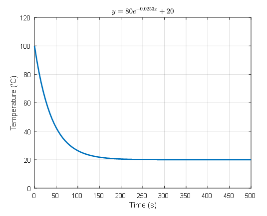
Figure 1. Cooling curve of an object using Newton's cooling law
Changes in salt concentration over time
When we were in elementary school, the problem of salt concentration in salt water was so difficult.
When solving problems with salt water in elementary school, the problem was to mix the salt water and adjust the concentration of the mixed salt water.
However, rather than mixing two cups of salt water and checking the concentration, what if we continuously pour a certain concentration of salt water into a water tank that originally contained pure water and observe the concentration of salt water over time?
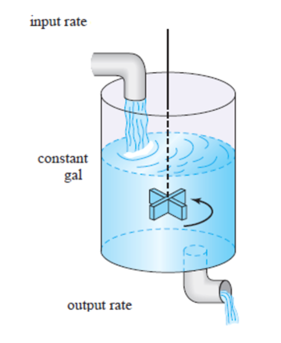
Figure 2. A situation where a tank with water is gradually mixed with salt water
Image source: Solution to the ODE-mixing tank problem using artificial neural networks, Aaron U Aquino & Elmer Dadios, 2015
Let’s consider continuously adding salt water with a concentration of 0.5 kg/L to a 1000 liter water tank containing only water.
Our goal is to fill the water tank with water of 0.5 kg/L concentration, and we want to maintain the water level of the tank.
To do this, let’s assume that we add 10 liters of 0.5 kg/L salt water to the tank every minute and remove 10 liters of water from the tank every minute.
Here, we will assume that we keep stirring the water in the tank so that the salt is evenly mixed.
This problem can be solved using differential equations. Let’s call the amount of salt in the water tank $x(t)$.
Then, the rate of change of salt in the water tank with respect to time will be $dx/dt$.
Also, the rate of change of salt per unit time is the difference between the rate of incoming salt and outgoing salt. Therefore,
\[\frac{dx}{dt}=\text{rate in }-\text{ rate out}\]can be written.
The incoming salt is 10L per minute, and the amount of salt is 0.5kg/L, so a total of 5kg of salt enters per minute.
The amount of outgoing water is 10L per minute, and since the water level is kept constant at 1000L, we can consider that 1/100 of the current salt amount is flowing out per minute. Therefore,
\[\frac{dx}{dt}=5-\frac{x}{100}\]We can solve this equation using separation of variables.
\[\frac{dx}{500-x}=\frac{dt}{100}\]Integrating both sides,
\[\Rightarrow -\ln|500-x| = \frac{t}{100}+C\]Thus,
\[500-x = Ce^{-0.01t}\]Using the initial condition $x(0)=0$,
\[\Rightarrow x(t) = 500-500 e^{-0.01t}\]
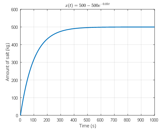
Figure 3. The solution curve of mixing problem