Matrices are Linear Transformations.
For any vectors $\vec a$ and $\vec b$, and any scalar $c$, a transformation $T$ is a linear transformation if it satisfies the following two conditions:
\[T(\vec a + \vec b) = T(\vec a)+T(\vec b)\] \[T(c \vec a) = c T(\vec a)\]Therefore, according to the properties of linear transformations mentioned above, for any vector
\[\left[\begin{array}{c} x\\ y\end{array}\right]\]the following holds:
\[T \left ( \begin{bmatrix}x \\ y \end{bmatrix} \right ) = T\left ( x \begin{bmatrix}1 \\ 0 \end{bmatrix} + y \begin{bmatrix}0 \\ 1 \end{bmatrix} \right ) = x T \left ( \begin{bmatrix}1 \\ 0 \end{bmatrix} \right ) + y T\left ( \begin{bmatrix}0 \\ 1 \end{bmatrix} \right )\]One thing to note here is that the original basis vectors are denoted as $\hat{i}$ and $\hat{j}$:
\[\hat i = \begin{bmatrix}1 \\ 0 \end{bmatrix}\] \[\hat j = \begin{bmatrix}0 \\ 1 \end{bmatrix}\]When we define new basis vectors as $\hat i_{new}$ and $\hat j_{new}$, we have:
\[\hat i_{new} = T\left ( \begin{bmatrix}1 \\ 0 \end{bmatrix} \right )\] \[\hat j_{new} = T\left ( \begin{bmatrix}0 \\ 1 \end{bmatrix} \right )\]If $T$ is a linear transformation, then the vector $\begin{bmatrix}x \ y \end{bmatrix}$ must be expressed as a linear combination of $\hat i_{new}$ and $\hat j_{new}$, where $\hat i_{new}$ is multiplied by $x$ and $\hat j_{new}$ is multiplied by $y$.
For example, if we use the matrix
\[A=\begin{bmatrix} 2 & -3 \\ 1 & 1 \end{bmatrix}\]to transform the vector
\[\vec x=\begin{bmatrix} 1 \\ 1 \end{bmatrix}\]we get:
\[A\vec x =\begin{bmatrix} 2 & -3 \\ 1 & 1 \end{bmatrix} \begin{bmatrix} 1 \\ 1 \end{bmatrix}=\begin{bmatrix} -1 \\ 2 \end{bmatrix}\]As shown in the video below, this value can be expressed as a combination of the new basis vectors, each multiplied by a coefficient of 1.
When we slide the slider in the applet all the way to the right, we get the following result:
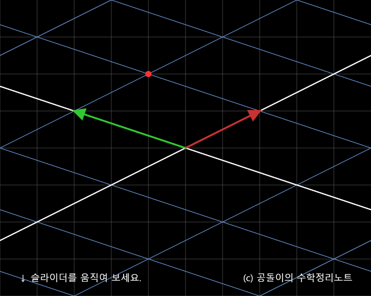
As we can see from the example, the red point representing the result of a linear transformation is expressed as -1, 2 times the original basis vectors, while the new basis vectors $\hat i_{new}$ and $\hat j_{new}$ after the linear transformation are expressed as 1, 1 times each.
In general, according to the fundamental theorem of linear algebra, linear transformations of vector spaces and matrices are fundamentally the same.
Visual Examples of Linear Transformations
One notable observation from the images and diagrams above is that geometrically, linear transformations maintain the shape of the grid as lines, and the spacing between the grid lines should be uniformly widened after the transformation.
Now that we have visualized various linear transformations (i.e., matrices) geometrically, we can confirm whether the grid lines maintain their linearity and uniform spacing after the transformation.