This post was written with reference to the lecture of Professor Nathan Kutz from the University of Washington, which can be found here.
Prerequisites
To better understand the contents of this post, it is recommended that you have knowledge of the following topics:
Introduction to Sturm-Liouville Theory
Sturm-Liouville theory 1 is a theory for obtaining solutions to second-order linear differential equations and understanding their properties. (In this post, we will refer to it as S-L theory for short.)
In particular, S-L theory starts with an attempt to obtain solutions to second-order linear differential equations from the perspective of operators, and to understand the characteristics of these solutions. The reason why this theory is significant is that even if a second-order differential equation is very complex, it can be interpreted differently if viewed from the perspective of S-L theory.
A differential equation of the form below, with a linear operator $L$, can be interpreted using Sturm-Liouville theory:
\[Lu=\mu r(x)u+f(x) % Equation (1)\]The following boundary conditions must be given:
\[\alpha_1 u(a)+\beta_1 \frac{du(a)}{dx}=0 % Equation (2)\] \[\alpha_2 u(b)+\beta_2 \frac{du(b)}{dx}=0 % Equation (3)\]Here, $\alpha$ and $\beta$ are constants that satisfy the following properties 2:
\[\alpha_1^2+\beta_1^2 >0 % Equation (4)\] \[\alpha_2^2+\beta_2^2 >0 % Equation (5)\]More specifically, the linear operator $L$ is given by:
\[Lu = -\frac{d}{dx}\left[p(x)\frac{du}{dx}\right]+q(x)u\]Here, $p(x)$, $q(x)$, and $r(x)$ must be functions greater than 0 on the interval $x\in[a,b]$.
Relationship with Second-order Linear Differential Equations
The form of equations that apply the Sturm-Liouville operator and the Sturm-Liouville theory may appear very unfamiliar.
However, if we apply this operator to solve equations, we can see that it is another way of writing a general second-order linear differential equation.
\[Lu=\mu r(x) u+f(x)\] \[\Rightarrow -\frac{d}{dx}\left[p(x)\frac{du}{dx}\right]+q(x)u=\mu r(x)u+f(x)\] \[\Rightarrow -\frac{dp}{dx}\frac{du}{dx}-p(x)\frac{d^2u}{dx^2}+(q(x)-\mu r(x))u=f(x)\]If we just rearrange the terms,
\[\Rightarrow -p(x)u''-\frac{dp}{dx}u'+(q(x)-\mu r(x))u=f(x)\]We can easily see that this is the form of a general second-order linear differential equation.
In other words, the Sturm-Liouville problem can be thought of as a theory established to find solutions of second-order differential equations that satisfy the condition that $p(x),q(x),r(x)$ among general 2nd order linear differential equations are functions greater than 0 and satisfy certain boundary conditions.
However, the reason why the theory was established in the form of the original Sturm-Liouville equation is that many problems are given in the form of equations similar to the Sturm-Liouville equation.
The S-L operator is a self-adjoint operator.
I think unfamiliar concepts will continue to appear.
What is self-adjoint?
As mentioned in the article “Linear Operators and Function Spaces”, adjoint corresponds to the concept of transpose of a matrix in linear algebra.
Let’s review adjoint briefly.
Let’s define the inner product of functions $f(x)$ and $g(x)$ defined on $x\in [a, b]$ as follows.
\[\langle f, g\rangle = \int_{a}^{b}\overline{f(x)}g(x)dx\]Here, the notation $\overline{f(x)}$ means that the complex conjugate is taken for the function $f(x)$.
Then, the adjoint $L^\dagger$ of a linear operator $L$ must satisfy the following property.
\[\langle Lf, g \rangle=\langle f, L^\dagger g\rangle\]In other words, a self-adjoint operator refers to an operator for which $L^\dagger = L$ holds. Therefore, it must satisfy the following property:
\[\langle Lf, g\rangle = \langle f, Lg\rangle\]These operators are similar to the concept of symmetric matrices or Hermitian matrices in linear algebra.
Now let’s confirm that the S-L operator is a self-adjoint operator:
\[\langle Lf, g\rangle = \int_a^b\left(-\frac{d}{dx}\left[p(x)\overline{f'}\right]+q(x)\overline f\right)g\ dx\] \[= \int_a^b -\frac{d}{dx}\left[p(x)\overline{f'}\right]g +q(x)\overline f g\ dx\]By using partial integration:
\[\Rightarrow -\left[p(x)\overline{f'}g\right]_a^b+\int_a^b\left(p(x)\overline{f'}g' + q(x)\overline f g\right)dx\]Similarly:
\[\langle f, Lg\rangle = \int_a^b\overline f\left(-\frac{d}{dx}\left[p(x)g'\right]+q(x)g\right)dx\]By using partial integration again:
\[=-\left[\overline{f} p(x)g'\right]_a^b+\int_a^b\left(\overline{f'}p(x)g'+\overline f q(x)g\right)dx\]Therefore, we need to check if $\langle Lf, g\rangle=\langle f, Lg\rangle$.
\[\langle Lf, g\rangle-\langle f, Lg\rangle = \left(-\left[p(x)\overline{f'}g\right]_{a}^{b}+\int_{a}^{b}\left(p(x)\overline{f'}g' + q(x)\overline f g \right)dx\right)\\-\left(-\left[\overline{f} p(x)g'\right]_{a}^{b}+\int_{a}^{b}\left(\overline{f'}p(x)g'+\overline f q(x)g \right)dx\right)\] \[=-\left[p(x)\overline{f'}g\right]_{a}^{b}+\left[\overline{f} p(x)g'\right]_{a}^{b}\] \[=-\left[p(x)\overline{f'}g-p(x)\overline{f}g'\right]_{a}^{b}\] \[=\left[p(x)W(\overline{f}, g)\right]_{a}^{b}\]Here, $W$ represents the Wronskian.
If we think carefully, $W(\overline{f},g)$ is always zero when $x=a$ or $x=b$. This is because if we express the boundary conditions of equation (2) for functions $\overline{f}$ and $g$ in matrix form, we get the following:
\[\begin{bmatrix}\overline{f(a)} &\overline{f'(a)}\\g(a) & g'(a)\end{bmatrix}\begin{bmatrix}\alpha_1 \\ \beta_1\end{bmatrix}=\begin{bmatrix}0 \\0\end{bmatrix}\]If the matrix on the left side of the above equation has an inverse, then both $\alpha_1$ and $\beta_1$ become zero, violating the condition in equation (4). Moreover, if both $\alpha_1$ and $\beta_1$ are zero, the boundary condition becomes meaningless, so $W(\overline{f},g)$ must be zero. The same method holds for $b$.
Therefore, we can see that $\langle Lf, g\rangle-\langle f, Lg\rangle = 0$.
Thus, we can conclude that the S-L operator $L$ is a self-adjoint operator.
Eigenvalue Problem in Sturm-Liouville Theory
Before dealing with the eigenvalue and eigenfunction problem of the S-L operator, let us define the inner product operation as follows for complex functions $f(x)$, $g(x)$, and $r(x)$ defined on the interval $[a,b]$.
\[\langle f, g \rangle_r=\int_{a}^{b}r(x)\overline{f(x)}g(x)dx\]Here, $r(x)$ is called the weighting function. In many cases, $r(x)=1$, but to include general cases where this is not the case, it is good to define the inner product in the above form. Let us write the inner product of functions with $r(x)=1$ as follows.
\[\langle f, g \rangle=\int_{a}^{b}\overline{f(x)}g(x)dx\]Also, to express orthogonality more easily, let us consider the Kronecker Delta function notation as follows.
\[\langle u_n, u_m\rangle_r=\delta_{mn}\]Here, $\delta_{mn}$ denotes a function that is equal to 1 only when $m=n$, and is equal to 0 otherwise.
Now, let us consider the S-L operator $L$ and the following equation.
\[Lu_n=\lambda_nr(x) u_n\]Here, $u_n$ is a function of $x$ and can be considered as an eigenfunction corresponding to the eigenvalue $\lambda_n$.
The right-hand side of this equation is given in the form multiplied by $r(x)$ to match the form of the right-hand side of the equation given in the original Sturm-Liouville theory.
Meanwhile, as mentioned earlier, we confirmed that the Sturm-Liouville operator is a self-adjoint operator. The self-adjoint operator can be thought of as an extension of the concept of Hermitian matrices in linear algebra, as briefly mentioned before.
In the eigenfunction expansion post, we introduced Hermitian matrices, and the most important characteristic of Hermitian matrices was that their eigenvalues are all real numbers, and the eigenvectors corresponding to different eigenvalues are all orthogonal.
Similarly, the self-adjoint operator also has eigenvalues and eigenvectors. Moreover, the eigenvalues of a self-adjoint operator are all real numbers, and if the eigenvalues are distinct, then the eigenvectors are orthogonal.
However, can we guarantee that all eigenvalues of the S-L operator are distinct, then all the eigenfunctions of the S-L operator can be orthogonal?
The answer is “yes”. If the S-L operator satisfies the conditions of Equations (2) through (5), all eigenvalues are distinct, and the eigenvectors are orthogonal. This can be proven through Sturm’s separation theorem, Sturm’s comparison theorem, and Sturm’s oscillation theorem. However, because of the author’s lack of mathematical knowledge, we will skip the proof.
By combining the contents so far and considering that the S-L operator is a self-adjoint operator and all eigenvalues are distinct, we can know that the S-L operator has the following properties:
- The eigenvalues of the S-L operator are all real numbers and can be arranged in the following order:
- The corresponding eigenfunctions to the above eigenvalues are all real functions and are orthogonal to each other as follows. For different eigenfunctions $y_n$, $y_m$ defined on the interval $[a,b]$,
- Based on the properties of the second eigenfunction, the eigenfunctions are a set of orthonormal basis for the Hilbert space ($L^2([a,b],w(x)dx)$), a function space that enables functions to be interpreted as points in an infinite-dimensional space.
The essential point is that the eigenfunctions of the S-L operator constitute an orthonormal basis for the Hilbert space.
\[u=\sum_{n=1}^{\infty}c_nu_n\]Using the same method, the forcing function $f(x)$ in equation (1) can also be expressed as a linear combination of eigenfunctions. This method is not much different from what we saw in the eigenfunction expansion article. The only difference is that we are applying it to the Sturm-Liouville problem this time.
To apply the orthogonality of eigenfunctions, $\langle u_n,u_m\rangle_r=\delta_{nm}$, let us consider the expression obtained by dividing $f(x)$ by $r(x)$ instead of trying to find $f(x)$. Let’s consider the following equation:
\[\frac{f(x)}{r(x)}=\sum_{n=1}^{\infty}b_n u_n\]To determine the value of $b_n$, let’s take the inner product as follows:
\[\left\langle\frac{f(x)}{r(x)}, u_m\right\rangle_r=\left\langle\sum_{n=1}^\infty b_nu_n, u_m \right\rangle_r\] \[\Rightarrow \int_{a}^{b}r(x)\left[\frac{f(x)}{r(x)}\right]u_m dx= \int_{a}^{b}r(x)\left(\sum_{n=1}^{\infty}b_nu_n\right)u_m dx\]When summation is taken in the right-hand side of the equation, the relationship $\langle u_n,u_m\rangle_r=\delta_{nm}$ applies, which means that $\langle u_n,u_m \rangle_r = 1$ only when $n=m$, and 0 for all other cases. Therefore,
\[\Rightarrow \int_{a}^{b}f(x)u_mdx=b_m\]That is, $b_n$ can be calculated as follows:
\[b_n=\langle f, u_n\rangle\]Returning to the eigenfunction expansion of the solution function, we can express $u$ in equation (1) using a linear combination of eigenfunctions as follows:
\[Lu=\mu r(x)u+f(x)\] \[\Rightarrow L\left(\sum_{n=1}^{\infty}c_nu_n\right)=\mu r(x)\left(\sum_{n=1}^{\infty}c_nu_n\right)+f(x)\]Since the operator $L$ is a linear operator, we can move the summation inside, resulting in:
\[\Rightarrow \left(\sum_{n=1}^{\infty}c_n L u_n\right)=\mu r(x)\left(\sum_{n=1}^{\infty}c_nu_n\right)+f(x)\]Here, $Lu_n$ can also be written using the eigenvalues.
\[\Rightarrow \left(\sum_{n=1}^{\infty}c_n \lambda_n r(x)u_n \right)=\mu r(x)\left(\sum_{n=1}^{\infty}c_nu_n\right)+f(x)\]Taking the inner product operation for $u_m$ here,
\[\Rightarrow \sum_{n=1}^{\infty}c_n\lambda_n \langle r(x)u_n, u_m\rangle=\mu\sum_{n=1}^{\infty}c_n\langle r(x)u_n, u_m\rangle + \langle f, u_m\rangle\] \[\Rightarrow \sum_{n=1}^{\infty}c_n\lambda_n \langle u_n, u_m\rangle_r=\mu\sum_{n=1}^{\infty}c_n\langle u_n, u_m\rangle_r + \langle f, u_m\rangle\] \[\Rightarrow c_m\lambda_m = \mu c_m + b_m\]Moving $\mu c_m$ on the right-hand side to the left and slightly rearranging the equation yields,
\[(\lambda_n-\mu)c_n = b_n, \quad n=1,2,3,\cdots\]Ultimately, our goal is to find $c_n$ to express the solution function. The solution exists only when $c_n$ exists appropriately. Therefore, from the above equation, we can determine the form of the existence of the solution according to the following conditions.
- Case 1: $\mu\neq \lambda_n$
-
Case 2: $\mu = \lambda_n, b_n\neq 0$, the solution does not exist.
-
Case 3: $\mu=\lambda_n, b_n=0$, not unique (if the null space is not a zero vector)
Since most cases follow Case 1, the solution function can be expressed as follows.
\[u(x)=\sum_{n=1}^{\infty}\frac{\langle f, u_n\rangle}{\lambda_n-\mu}u_n(x)\]Example Problem
Second-order Inhomogeneous Differential Equation
Solve the following second-order inhomogeneous differential equation from the perspective of Sturm-Liouville theory:
\[\frac{d^2u}{dx^2}+2u=-x\]Here, $x\in[0,1]$ and the boundary conditions are as follows:
\[u(0)=0\] \[u(1)+u'(1)=0\]Solution
We can express this problem in Sturm-Liouville form as follows:
\[-\frac{d^2}{dx^2}u=2u+x\]In other words, from the perspective of the original equation (1) and equation (6), we can see that this is a very simple Sturm-Liouville problem with $p(x)=1$, $q(x)=0$, $r(x)=1$, $\mu=2$, and $f(x)=x$.
Note that from another perspective, we could also view this as a Sturm-Liouville problem with $\mu=0$ and $q(x)=-2$, but this is just a matter of perspective.
The eigenvalue problem for this equation is as follows:
\[-\frac{d^2u_n}{dx^2}=\lambda_n u_n\]The general solution to this eigenvalue problem is:
\[u_n=c_1 \sin\sqrt{\lambda_n}x + c_2 \cos\sqrt{\lambda_n}x\]To satisfy the boundary condition $u_n(0)=0$, we need $c_2=0$, so the eigenfunction can be written as:
\[u_n=c_1\sin\sqrt{\lambda_n}x\]To satisfy the other boundary condition, $u_n(1)+u’_n(1)=0$, we need to find $u’(x)$:
\[u'(x)=\sqrt{\lambda_n}c_1\cos\sqrt{\lambda_n}x\]Thus, $u_n(1)+u’_n(1)$ becomes:
\[u_n(1)+u'_n(1)=c_1\sin\sqrt{\lambda_n}+\sqrt{\lambda_n}c_1\cos\sqrt{\lambda_n}=0\]We cannot allow $c_1$ to be 0 (otherwise, we would get a trivial solution), so the eigenvalues must satisfy the following condition:
\[\sin\sqrt{\lambda_n}+\sqrt{\lambda_n}\cos\sqrt{\lambda_n}=0\]Here, if we divide both sides by $\cos\sqrt{\lambda_n}$,
\[\Rightarrow \sqrt{\lambda_n}+\tan\sqrt{\lambda_n}=0\]the values of $\lambda_n$ that satisfy this equation are the eigenvalues.
To obtain the solutions to the above equation, we need to find the intersection points of the functions $y=\tan(x)$ and $y=-x$. Obtaining the solution using conventional methods is difficult, but using a computer, we can obtain the following results:
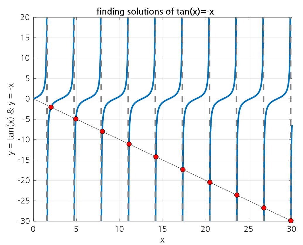
Figure 1. Solutions to tan(x)+x=0
Then, we can see that the above values correspond to $\sqrt{\lambda_n}\text{ for } n = 1,2,\cdots$.
At this point, the normalized eigenfunctions $u_n$ that correspond to each eigenvalue can be modified to satisfy $\langle u_n, u_n \rangle = 1$ as follows:
\[u_n = \frac{\sqrt{2}}{(1+\cos^2\sqrt{\lambda_n})^{1/2}}\sin\sqrt{\lambda_n}x\quad\quad n=1,2,\cdots\]Therefore, we can express $f(x)$ and $u(x)$ using these eigenfunctions.
To do this, first let’s calculate $b_n$:
\[b_n = \langle f, u_n\rangle = \int_{0}^{1}\left(\frac{\sqrt{2}}{(1+\cos^2\sqrt{\lambda_n})^{1/2}}x\sin\sqrt{\lambda_n}x \right)dx=\frac{2\sqrt{2}\sin\sqrt{\lambda_n}}{\lambda_n(1+\cos^2\sqrt{\lambda_n})^{1/2}}\]Then, we have:
\[f(x)=4\sum_{n=1}^{\infty}\frac{\sin\sqrt{\lambda_n}\sin\sqrt{\lambda_n}x}{\lambda_n(1+\cos^2\sqrt{\lambda_n})}\]and
\[u(x)=4\sum_{n=1}^{\infty}\frac{\sin\sqrt{\lambda_n}\sin{\sqrt{\lambda_n}x}}{\lambda_n(\lambda_n-2)(1+\cos^2\sqrt{\lambda_n})}\]These results may seem somewhat complex, but they can be easily understood by watching the following video:
Through the method of solving a general inhomogeneous differential equation, $u(x)$ can be found to be:
\[u(x)=0.82761\sin(\sqrt{2}x)-\frac{x}{2}\]By comparing this expression to $u(x)$ expressed as a linear combination of the eigenfunctions found above, it can be seen that it converges to the same result.
Figure 2. The process of approximating $u(x)$ using a linear combination of eigenfunctions.
What’s even more amazing is that the function $f(x)=x$ can also be expressed as a linear combination of eigenfunctions.
This concept is further extended to the Fourier series. The Fourier series expresses an arbitrary periodic function as a sum of trigonometric functions.
The reason why the Fourier series can work mathematically flawlessly lies in this deep background knowledge.
Figure 3. The process of approximating $f(x)$ using a linear combination of eigenfunctions.
Fourier Series
The Fourier series can be considered as a series that appears in the process of solving the Sturm-Liouville problem below.
Consider the following simple linear operator:
\[L=-\frac{d^2}{dx^2}\]This operator is assumed to be the case for $p(x)=1$ and $q(x)=0$ in equation (6), and for $r(x)=1$. Consider the following eigenvalue problem:
\[Lu_n=\lambda_n u_n\]where $n=1,2,\cdots,\infty$.
Also, let’s give the boundary value condition as follows:
\[u(0)=u(\pi)=0\]The solution to this eigenvalue problem can be simply given as a combination of sine waves as follows:
\[u_n(x)=c_1\cos(\sqrt{\lambda_n}x)+c_2\sin(\sqrt{\lambda_n}x)\]If we substitute $u(0)=0$ among the boundary conditions,
\[u_n(0)=c_1=0\]and if we substitute $u(\pi)=0$ among the boundary conditions,
\[u_n(\pi)=c_2\sin(\sqrt{\lambda_n}\pi)=0\]must be satisfied. Since $c_2$ must be a non-zero value for the eigenvector of the solution to the eigenvalue problem to be a non-trivial solution, the eigenvalue is
\[\sqrt{\lambda_n}=n\]and the eigenvector is
\[u_n=\sin(nx)\]To make $\langle u_n,u_n\rangle = 1$ here, let’s check the following.
\[\langle u_n, u_n\rangle = \int_{0}^{\pi}\sin(nx)\sin(nx)dx\] \[=\int_{0}^{\pi}\frac{-\cos(2nx)+\cos(0)}{2}dx\] \[=\frac{1}{2}\int_{0}^{\pi}\cos(0)-\cos(2nx)dx\] \[=\frac{1}{2}\left(x-\frac{1}{2n}\sin(2nx)\right)_{0}^{\pi}\] \[=\frac{\pi}{2}\]Therefore, to make $\langle u_n,u_n\rangle = 1$, let’s modify the form of the eigenfunction as follows.
\[u_n=\sqrt{\frac{2}{\pi}}\sin(nx)\]Here, $n=1,2,\cdots, \infty$.
Now let’s assume that we solve the following nonhomogeneous differential equation using the operator $L$.
\[Lu=f(x)=x,\quad x\in[0,\pi]\]Similarly, let’s assume that the boundary condition is given as $u(0)=u(\pi)=0$.
According to the result of equation (31), $f(x)=x$ can be expressed as a linear combination of eigenfunctions as follows.
\[f(x)=\sum_{n=1}^{\infty}b_n u_n=\sum_{n=1}^{\infty}b_n \sqrt{\frac{2}{\pi}}\sin(nx)\]And $b_n$ can be calculated as shown in equation (35).
\[b_n=\langle f, u_n\rangle = \int_{0}^{\pi}x\sqrt{\frac{2}{\pi}}\sin(nx)dx\] \[=\sqrt{\frac{2}{\pi}}\int_{0}^{\pi}x\sin(nx)dx\] \[=\sqrt{\frac{2}{\pi}}\left(-\frac{1}{n}x\cos(nx)\Big|_{0}^{\pi}+\int_{0}^{\pi}\frac{1}{n}\cos(nx)dx\right)\] \[=\sqrt{\frac{2}{\pi}}\left(-\frac{1}{n}\pi\cos(n\pi)-\frac{1}{n}\cdot\frac{1}{n}(\sin(nx))\Big|_{0}^{\pi}\right)\] \[=\sqrt{\frac{2}{\pi}}\left(-\frac{1}{n}\pi(-1)^n\right)\]Therefore, $f(x)=x$ can be expressed as a linear combination of trigonometric functions as follows.
\[f(x)=x=\sum_{n=1}^{\infty}\sqrt{\frac{2}{\pi}}\left(-\frac{1}{n}\pi(-1)^n\right)\sqrt{\frac{2}{\pi}}\sin(nx)\] \[=\sum_{n=1}^{\infty}\frac{2}{\pi}\left(-\frac{1}{n}\pi(-1)^n\right)\sin(nx)\] \[=\sum_{n=1}^{\infty}-\frac{2}{n}(-1)^n\sin(nx)\]
Figure 4. The process of approximating $f(x)=x$ using linear combinations of eigenfunctions of the operator $L=-u''$ (equivalent to Fourier sine series).
Bessel Differential Equation
Another charm of Sturm-Liouville theory is when it is applied to various special differential equations.
By showing that several special differential equations that are difficult to solve by hand can be expressed in the Sturm-Liouville form, it becomes possible to understand the characteristics of the solutions, although obtaining the solutions themselves may still be difficult.
For instance, the Bessel equation is of the following form:
\[x^2y''+xy'+(x^2-\nu^2)y=0\]The Bessel equation can be expressed in Sturm-Liouville form as follows:
\[(xy')'+\left(x-\frac{\nu^2}{x}\right)y=0\]Legendre Differential Equation
The Legendre equation is of the following form:
\[(1-x^2)y''-2xy'+\nu(\nu+1)y=0\]The Legendre equation can also be expressed in the following form:
\[((1-x^2)y')'+\nu(\nu+1)y=0\]