Reasons for the Need of Hilbert Transform
To explain the reasons for the need of Hilbert transform, it is important to understand the role of Hilbert transform and the results that can be obtained by performing the role. Firstly, the role of Hilbert transform is to act as a kind of linear filter that maintains the amplitude of a signal while shifting the phase by $-\frac{\pi}{2}$ (or by $\frac{\pi}{2}$ for negative frequencies).
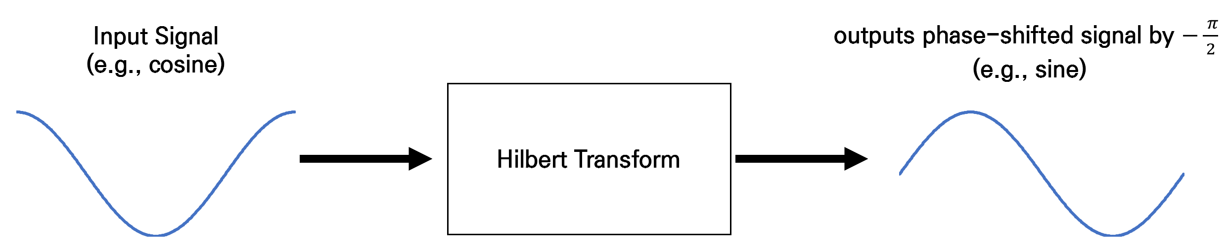
Figure 1. Hilbert transform maintains the amplitude of the original signal and shifts the phase by -90'.
Characteristics of Hilbert Transform
The Hilbert transform filter is a filter that does not change in magnitude at all frequencies (all-pass filter), but only changes the phase by +90 degrees for negative frequencies and -90 degrees for positive frequencies. In other words, if a cosine signal of frequency $\omega$ is input, the output will always be a sine signal of frequency $\omega$.
Therefore, by defining Hilbert transform, any real-valued signal can be phase-shifted by $-\frac{\pi}{2}$ or $\frac{\pi}{2}$, allowing the analysis of amplitude and phase to be easier by extending the real-valued signal to the complex plane. That is, for a real-valued signal $x(t)$ and a Hilbert-transformed signal $\hat{x}(t)$, we can consider a signal extended to the complex plane as $x_p(t)=x(t)+j\hat{x}(t)$.
For example, if the signal $x(t)$ is $cos(\omega_0t+\theta)$, we can consider the signal $x_p(t)=cos(\omega_0t+\theta)+j sin(\omega_0t+\theta)$ in the complex plane. As is well known, the signal $x_p(t)$ can be expressed as $x_p(t)=e^{j(\omega_0t+\theta)}$, and the phase of this signal can be easily calculated using the complex plane and Euler’s formula. This method of extending a real-valued signal to the complex plane and interpreting it is called “deriving the analytic signal.”
While this analysis method applies only to special cases such as $x(t)=cos(\omega_0t+\theta)$, extending a real-valued signal to the complex plane and deriving the analytic signal is a very significant process that can be applied to any real-valued signal.
Derivation of Hilbert Transform
Hilbert transform acts as a filter that changes only the phase while maintaining the amplitude. Therefore, it can be considered as an all-pass filter, and the transfer function that satisfies the characteristics of Hilbert transform is as follows.
\[|H(f)| = 1\]and
\[\angle H(f) = \begin{cases} \pi/2, & \text{for $f < 0$} \\ -\pi/2, & \text{for $f>0$} \end{cases}\]So, we can generalize $H(f)=-j\times sgn (f)$1. Therefore, the impulse function $h(t)$, which is the transformation kernel, can be obtained by taking the inverse Fourier Transform of $H(f)=-j\times sgn(f)$.
PROOF Derivation of the Hilbert transform kernel
In this case, we can approximate $sgn(f)$ as follows.
\[sgn(f) \rightarrow G(f;\alpha) = \begin{cases}e^{-\alpha f}, & \text{for $f > 0$} \\-e^{\alpha f}, & \text{for $f < 0$} \end{cases}\]It can be observed that $G(f;\alpha)$ becomes very close to $sgn(f)$ as $\alpha\rightarrow 0$.
Therefore, during the derivation process, let’s consider the inverse Fourier transform of $G(f;\alpha)$ and then think about the shape of $g(t)$ as $\alpha\rightarrow 0$.
Hence,
\[h(t)=-j\lim_{\alpha\rightarrow 0}g(t;\alpha)\]and $g(t;\alpha)$ can be derived as follows.
\[g(t;\alpha) = \int_{-\infty}^{\infty}G(f;\alpha) e^{j2\pi ft}df\] \[= \int_{-\infty}^{0}-e^{\alpha f}e^{j2\pi ft}df + \int_{0}^{\infty}e^{-\alpha f}e^{j2\pi ft}df\] \[= \int_{-\infty}^{0}-e^{\alpha f+j2\pi ft}df + \int_{0}^{\infty}e^{-\alpha f+j2\pi ft}df\] \[= - \frac{1}{(\alpha + j 2\pi t)}\left|e^{(\alpha + j 2\pi t)f}\right|_{-\infty}^{0} +\frac{1}{(-\alpha + j 2\pi t)}\left|e^{(-\alpha + j 2\pi t)f}\right|_{0}^{\infty}\] \[= - \frac{1}{(\alpha + j 2\pi t)} (1-0) +\frac{1}{(-\alpha + j 2\pi t)} (0-1)\] \[= -\frac{1}{(\alpha + j 2\pi t)} - \frac{1}{(-\alpha + j 2\pi t)}\] \[=\frac{1}{(\alpha -j 2\pi t)} - \frac{1}{(\alpha + j 2\pi t)} = \frac{j4\pi t}{\alpha ^2 + (2\pi t)^2}\]Thus,
\[h(t) = -j \lim_{\alpha \rightarrow 0}g(t;\alpha) = -j\lim_{\alpha \rightarrow 0}\frac{j4\pi t}{\alpha ^2 + (2\pi t)^2}\] \[= -j \frac{j4\pi t}{4\pi ^2 t^2} = -j \frac{j}{\pi t} = \frac{1}{\pi t}\]As a general rule, the output function $y(t)$ for an input function $x(t)$ can be expressed in terms of the impulse response $h(t)$ of the system as:
\[y(t)=x(t)\otimes h(t)=\int_{-\infty}^{\infty}{x(t)h(t-\tau)d\tau}\]In the case of the Hilbert transform, if we denote the output as $\hat{x}(t)$ instead of $y(t)$, the following relation holds:
\[\hat{x}(t) = \int_{-\infty}^{\infty}x(t) \frac{1}{\pi(t-\tau)d\tau}\] \[=\frac{1}{\pi}\int_{-\infty}^{\infty}x(t) \frac{1}{t-\tau}d\tau\]Properties of the Hilbert Transform
The Hilbert transform of a signal $x(t)$, denoted as $\hat{x}(t)$, has the following properties.
Double Application of the Hilbert Transform
Applying the Hilbert transform twice to a signal results in the reversal of its sign. This is because it introduces a phase shift of $-\pi$ or $\pi$. Mathematically, this can be expressed as:
\[\left(H(f)\right)^2 = \begin{cases}j \times j = -1, & \text{for $f < 0$} \\(-j)\times (-j) = -1, & \text{for $f > 0$}\end{cases}\]In other words,
\[\hat{\hat{x}}(t) = -x(t)\]Hilbert transform for trigonometric functions
-
$x(t) = \cos(2\pi f_0 t) \Leftrightarrow \hat{x}(t) = \sin(2\pi f_0 t)$
-
$x(t) = \sin(2\pi f_0 t) \Leftrightarrow \hat{x}(t) = -\cos(2\pi f_0 t)$
-
$x(t) = \exp(j2\pi f_0 t)$
$x(t)$ and $\hat{x}(t)$ have the same amount of energy (or power).
This can be derived from Parseval’s theorem. Let’s denote the Fourier transform of $\hat{x}(t)$ as $\hat{X}(f)$. Since $\hat{X}(f) = -j \times \text{sgn}(f)X(f)$, we have:
\[\left|\hat{X}(f)\right| = \left|X(f)\right|\]This implies that the energy or power of $x(t)$ and $\hat{x}(t)$ are equal, as shown by the following Parseval’s theorem:
\[\int x^2(t) dt = \int \left|X(f)\right|^2 df\]$x(t)$ and $\hat{x}(t)$ are orthogonal functions.
In other words, the inner product of $x(t)$ and $\hat{x}(t)$ is zero, i.e.,
\[\int_{-\infty}^{\infty}x(t)\hat{x}(t)dt = 0\]This can also be proved using Parseval’s theorem. Applying the general Parseval’s theorem for complex signals, the inner product can be expressed as:
\[\int_{-\infty}^{\infty}X(f)\hat{X}^*(f) df\] \[=\int_{-\infty}^{\infty}X(f)\space j \space \text{sgn}(f) X^*(f)df\] \[=\int_{-\infty}^{\infty} j\space \text{sgn}(f) \left|X(f)\right|^2 df = 0\]This is because $\text{sgn}(f)$ is a symmetric function with respect to 0.
Bedrosian identity (☆)
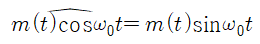
Let’s consider two signals, $c(t)$ and $m(t)$, whose frequency spectra do not overlap. In this case, we can say that $m(t)$ is a low-pass filter and $c(t)$ is a high-pass filter, and the following equation holds:
In other words, when a signal is amplitude modulated with a high frequency $f_0$, with the modulating signal denoted as $m(t)$ and the carrier signal denoted as $c(t)$, the following equations hold:
Envelope of a Signal
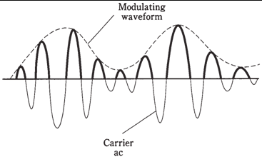
Figure 2. Illustration of the envelope of a signal.
(Source: http://www.expertsmind.com/CMSImages/2091_Detection%20of%20AM%20signals.png)
The Hilbert transform can be used to obtain the envelope of an amplitude modulated signal using the Bedrosian identity.
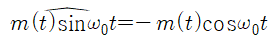
In other words, when the low-pass filter $m(t)$ is amplitude modulated with a high frequency $f_0$, and the carrier signal is denoted as $c(t) = \cos(\omega_0 t)$, the AM signal is given by $x(t) = m(t)c(t)$.
In this case, the Hilbert transform of $x(t)$ can be represented as:
\[x_p(t) = x(t) +j \hat{x}(t)\]where
\[\hat{x}(t) = \sin (\omega_0 t)\]Thus,
\[x_p(t) = m(t) \cos(\omega_0 t) + j m(t) \sin (\omega_0 t) \notag\] \[=m(t) \exp(j\omega_0t)\]Therefore,
\[\left|x_p(t)\right| = \left|m(t) \exp(j\omega_0 t)\right| = \left|m(t)\right|\]which is the envelope of the AM signal.
-
The function sgn() outputs +1 for positive inputs and -1 for negative inputs. It is pronounced as ‘signum’. ↩