Prerequisites
To understand this post well, it is recommended to know the following:
Homogeneous Linear Second-Order Differential Equations
A second-order linear differential equation refers to a differential equation where the maximum order of the differential coefficient is 2, as shown below.
\[a(t)\frac{d^2x}{dt^2} + b(t)\frac{dx}{dt} + c(t)x(t) = g(t) % Equation (1)\]In this session, we will deal with a special case of a homogeneous second-order linear differential equation where $a(t)$, $b(t)$, and $c(t)$ are all constants and $g(t)=0$.
In other words, the form of the differential equation we want to handle is as follows.
\[a\frac{d^2x}{dt^2}+b\frac{dx}{dt}+cx(t) = 0 % Equation (2)\]Here, $a$ must not be 0.
Solution Using Linear Systems of Differential Equations
In fact, we have dealt with the solution to a second-order homogeneous linear differential equation before.
When we covered damped harmonic oscillation in the post Modeling with Systems of Differential Equations, we mentioned this solution.
The solution to a second-order homogeneous linear differential equation is to set the first-order differential coefficient $dx/dt$ as a new variable and solve it.
For a second-order homogeneous linear differential equation like Equation (2), we can think as follows.
If we define a new variable $y$ as follows:
\[y=\frac{dx}{dt} % Equation (3)\]then,
\[\frac{dy}{dt}=\frac{d}{dt}\left(\frac{dx}{dt}\right)=\frac{d^2x}{dt^2} % Equation (4)\]Therefore, Equation (2) can be written as follows.
\[a\frac{dy}{dt}+by+cx = 0 % 식 (5)\] \[\Rightarrow \frac{dy}{dt}=-\frac{b}{a}y-\frac{c}{a}x % 식 (6)\]Once again, if we solve the process as a system of differential equations for $x$ and $y$, it can be expressed as follows:
\[\begin{cases}\dfrac{dx}{dt}=y \\\\ \dfrac{dy}{dt}=-\dfrac{c}{a}x-\dfrac{b}{a}y\end{cases} % Equation (7)\]Therefore, the second-order homogeneous linear differential equation in Equation (2) can always be represented in the form of a matrix as follows:
\[\begin{bmatrix}dx/dt \\ dy/dt \end{bmatrix} = \begin{bmatrix}0 & 1 \\ -c/a & -b/a\end{bmatrix}\begin{bmatrix}x \\ y\end{bmatrix} % Equation (8)\]It is emphasized several times, but $a$ must not be zero in Equation (8).
From here, we can obtain the solution of the second-order homogeneous linear differential equation by solving Equation (8).
The significance of solving the system of linear differential equations
As we saw in the phase plane article, solving a system of linear differential equations to obtain the solution of a second-order homogeneous differential equation is the connecting link to use the eigenvalues and eigenvectors of the matrix in Equation (8).
Let’s try to find the eigenvalues and eigenvectors of the matrix in Equation (8).
If we try to find the characteristic equation of the matrix in Equation (8), it can be expressed as follows:
\[\text{det}\left(\begin{bmatrix}0-\lambda & 1 \\ -c/a & -\frac{b}{a}-\lambda \end{bmatrix}\right)\] \[=-\lambda\left(-\frac{b}{a}-\lambda\right)+\frac{c}{a}\] \[=\lambda^2 +\frac{b}{a}\lambda+\frac{c}{a}=0\]We can use the quadratic formula to find the solutions of the characteristic equation.
\[\lambda =\frac{-b/a\pm\sqrt{\left(b/a\right)^2-4(c/a)}}{2}\] \[=\frac{-b\pm\sqrt{b^2-4ac}}{2a}\]And if we find the eigenvectors, we can see that they are as follows:
\[v_1 = \begin{bmatrix}1\\-(b+\sqrt{b^2-4ac})/2a\end{bmatrix}=\begin{bmatrix}1\\ \lambda_1\end{bmatrix}\] \[v_2 = \begin{bmatrix}1\\-(b-\sqrt{b^2-4ac})/2a\end{bmatrix}=\begin{bmatrix}1\\ \lambda_2\end{bmatrix}\]Therefore, according to the general solution formula of the system of differential equations, if we write the solution as follows:
\[\begin{bmatrix}x(t)\\y(t)\end{bmatrix}=c_1e^{\lambda_1 t}\begin{bmatrix}1 \\ \lambda_1\end{bmatrix}+c_2e^{\lambda_2 t}\begin{bmatrix}1 \\ \lambda_2\end{bmatrix}\]Here, $c_1$, $c_2$ are arbitrary constants and $\lambda_{1,2}$ are
\[\lambda_{1,2}=\frac{-b\pm \sqrt{b^2-4ac}}{2a}\]When solving a second-order differential equation, we set $y=dx/dt$ and if we only take the $x(t)$ part of equation (16), it becomes the solution of the second-order differential equation.
Therefore, the solution $x(t)$ of the homogeneous linear second-order differential equation is as follows:
\[x(t)=c_1e^{\lambda_1 t}+c_2e^{\lambda_2 t}\]Example Problem
Since it can be difficult to understand with only theoretical explanations, let’s solve an example problem of a second-order homogeneous differential equation.
Let’s solve the following second-order homogeneous differential equation:
\[\frac{d^2x}{dt^2}-4\frac{dx}{dt}+3x(t) = 0 % Equation (13)\]To solve this problem, let’s convert the second-order differential equation into a system of first-order differential equations.
To do this, let’s consider the new variable $y(t)$ as follows:
\[y(t) = \frac{dx}{dt}\]Then, we can obtain the following relationship:
\[\frac{dy}{dt}=\frac{d^2x}{dt^2} = 4\frac{dx}{dt}-3x(t)\]Therefore, we can obtain the following system of first-order differential equations:
\[\begin{cases}\dfrac{dx}{dt} = y\\\\ \dfrac{dy}{dt}=-3x+4y\end{cases}\] \[\Rightarrow \begin{bmatrix}dx/dt \\ dy/dt\end{bmatrix} = \begin{bmatrix}0 & 1 \\ -3 & 4\end{bmatrix}\begin{bmatrix}x \\ y\end{bmatrix}\]Now, let’s find the eigenvalues and eigenvectors of the matrix in Equation (23).
According to the definition of eigenvalues and eigenvectors, if the eigenvector is $\vec{v}$ and the eigenvalue is $\lambda$, it must satisfy the following equation:
\[\begin{bmatrix}0 & 1 \\ -3 & 4 \end{bmatrix}\vec{v} = \lambda\vec{v}\]Moving all terms to the left-hand side, we get:
\[\begin{bmatrix}-\lambda & 1 \\ -3 & 4-\lambda\end{bmatrix}\vec{v} = 0\]To prevent $\vec{v}$ from becoming a zero vector, the matrix in Equation (25) must satisfy the following condition (also known as the characteristic equation).
\[det\left(\begin{bmatrix}0-\lambda & 1 \\ -3 & 4-\lambda\end{bmatrix}\right) = 0\] \[=\lambda(\lambda-4)+3\] \[=\lambda^2 - 4 \lambda + 3 = 0\]Therefore, the eigenvalues are
\[\lambda = 1 \text{ or } 3\]If we find the eigenvectors corresponding to each eigenvalue, using equation (25),
For $\lambda = 1$,
\[Equation(26) \Rightarrow\begin{bmatrix}0 -1 & 1 \\ -3 & 4-1 \end{bmatrix}\vec{v} = \lambda\vec{v}\] \[=\begin{bmatrix}-1 & 1 \\ -3 & 3\end{bmatrix}\begin{bmatrix}v_1 \\ v_2\end{bmatrix}\] \[=\begin{bmatrix}-v_1 + v_2 \\ -3 v_1 + 3v_2 \end{bmatrix}=\begin{bmatrix}0 \\ 0\end{bmatrix}\] \[\therefore \vec{v} = \begin{bmatrix}1 \\ 1\end{bmatrix}\]Also, for $\lambda = 3$,
\[Equation(26) \Rightarrow\begin{bmatrix}0 -3 & 1 \\ -3 & 4-3 \end{bmatrix}\vec{v} = 0\] \[= \begin{bmatrix}-3 & 1 \\ -3 & 1 \end{bmatrix}\begin{bmatrix}v_1 \\ v_2\end{bmatrix} = 0\] \[= \begin{bmatrix}-3 v_1& v_2 \\ -3v_1 & v_2 \end{bmatrix}\vec{v} = \begin{bmatrix}0 \\ 0\end{bmatrix}\] \[\therefore \vec{v} = \begin{bmatrix}1 \\ 3\end{bmatrix}\]Therefore, the general solution of equation (23) is
\[\begin{bmatrix}x(t) \\ y(t) \end{bmatrix} = c_1\begin{bmatrix}1 \\ 1\end{bmatrix}e^t + c_2 \begin{bmatrix}1 \\3 \end{bmatrix}e^{3t}\]Thus, the general solution of equation (19) is
\[x(t) = c_1e^t + c_2e^{3t}\]For reference, if we draw a phase plane for equation (23), it looks like the following. The thick black lines are the straight lines following the eigenvectors.
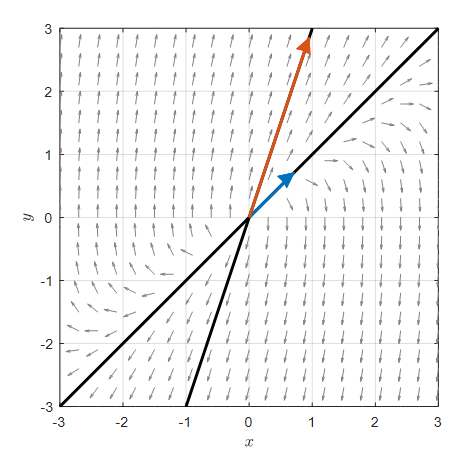
Figure 2. Phase plane for the system of differential equations in Equation (23). The thick black lines are the straight lines following the eigenvectors.