Non-negative Matrix Factorization(NMF)

Prerequisites

To understand this post, it is recommended that you have a good understanding of the following topics:

Although Independent Component Analysis may be difficult to understand, it is not necessary to fully understand it. However, it is recommended that you have a good understanding of Principal Component Analysis and Gradient Descent.

Definition of NMF

Non-negative Matrix Factorization (NMF) is an algorithm that decomposes a non-negative matrix $X$ into the product of two non-negative matrices $W$ and $H$.

This can be expressed mathematically as follows:

\[X = WH\]

The Meaning of W and H

Before discussing the meaning of $W$ and $H$, let’s think about what kind of matrix $X$ is that we want to decompose.

It may be helpful to think of $X$ as a dataset. If $X$ is an $m\times n$ matrix, then $m$ can be thought of as the number of observations and $n$ can be thought of as the dimension of each data sample vector.

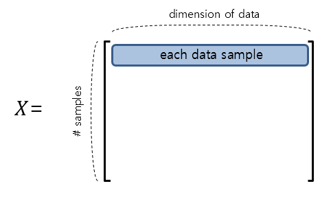
Figure 1. The shape of the data matrix $X$

On the other hand, the dimensions of $W$ and $H$ can be determined according to the user’s needs. Of course, the number of rows of $W$ and the number of columns of $H$ should be $m$ and $n$, respectively.

For example, if we want to decompose the original dataset $X$ using $p$ features, the dimensions of $W$ and $H$ will be determined as follows.

\[W\in \Bbb{R}^{m\times p}\] \[H\in \Bbb{R}^{p\times n}\]

When we decompose the data using NMF, we can consider the matrix H first. Each row of H becomes a feature, and each row of W represents the weight of how much each feature is mixed.

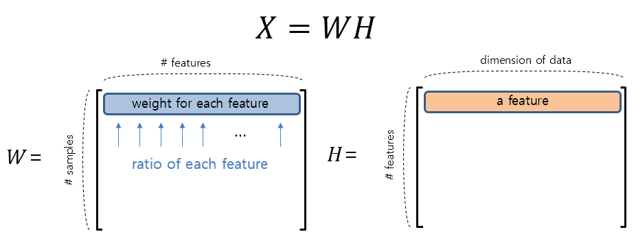
Figure 2. The shape of the decomposed matrix W and H using NMF and the meaning of each row in the matrices.

Why is NMF useful?

Non-negative data should be explained by non-negative features.

One reason NMF is useful is that the extracted features are all non-negative. Some of the data we deal with does not contain negative values. For example, in the image shown above, all the data are composed of pixel intensities, and there are no negative values among these values. Therefore, if we assume that the data are appropriately arranged features such as eyes, nose, mouth, and ears in a picture of a face, it is natural to assume that these features are all composed of non-negative values.

However, many matrix factorization methods such as SVD or dimensionality reduction methods such as factor analysis, principal component analysis, and cluster analysis do not have restrictions that extracted features should not be negative. Thus, there is no guarantee that non-negativity of the data will be preserved.

NMF can capture the independence of features well.

Another reason NMF is useful is that it can better reflect the structure of the data compared to factorization methods such as PCA or SVD. PCA and SVD guarantee orthogonality between features because the algorithms are designed that way. If we only explain PCA, it is a decomposition using eigenvectors of the covariance matrix, and it can be mathematically proven that the eigenvectors of the covariance matrix are always orthogonal because the covariance matrix is a symmetric matrix. (For a more detailed explanation, please refer to the articles on PCA and SVD.)

However, if the feature vectors become orthogonal to each other, they may not reflect the actual data structure of the dataset well. Let’s take a look at the differences between PCA and NMF through the following figure.

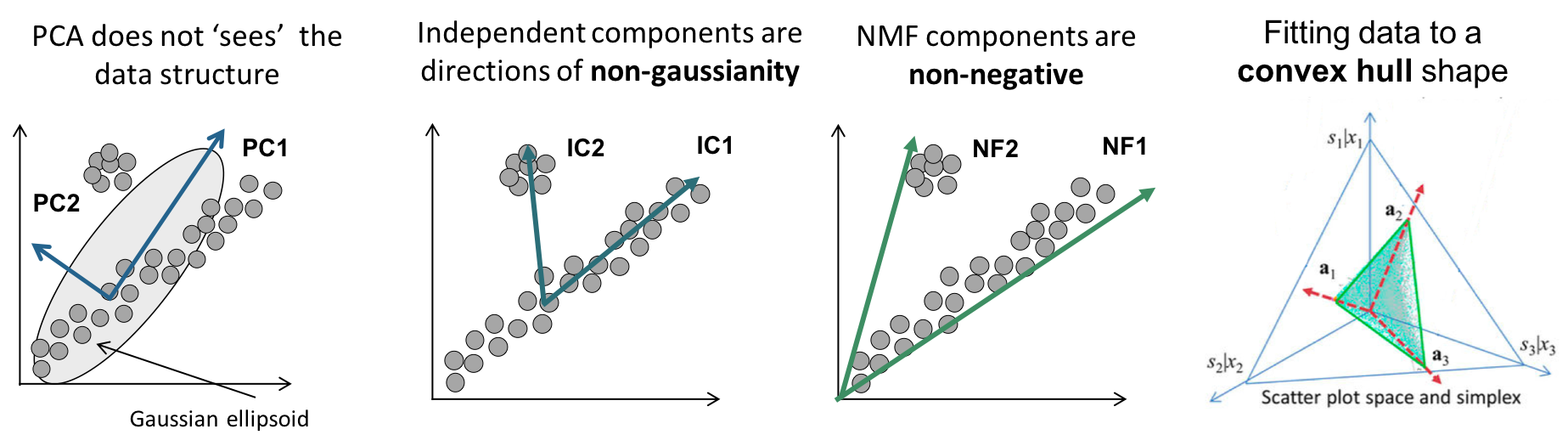
Figure 3. Geometrical interpretation of PCA and NMF
Image source

Necessary Pre-Techniques

Before we delve into how to obtain the results of NMF, namely $W$ and $H$, let us first understand some necessary pre-knowledge.

Trace Operator

Occasionally, we may only need the diagonal elements of a matrix. In particular, there are cases where only the trace component is needed. In such cases, the trace operator can be used.

In other words, the trace operator is defined as follows:

\[tr\left(\begin{bmatrix}a_{11} && a_{12} && a_{13} \\ a_{21} && a_{22} && a_{23}\\a_{31} && a_{32} && a_{33}\end{bmatrix}\right) = a_{11}+a_{22}+a_{33}\]

Here are some properties of the trace operator:

\[tr(A+B) = tr(A) + tr(B)\] \[tr(ABC) = tr(CAB) = tr(BCA)\]

Furthermore, the derivative (i.e., gradient) of a matrix with respect to a trace-containing product of two or more matrices is as follows:

These four equations will be useful when we derive the algorithm of NMF below, so let’s keep them in mind.

\[\nabla_X tr(AX) = A^T\] \[\nabla_X tr(X^TA) = A\] \[\nabla_X tr(X^TAX) = (A+A^T)X\] \[\nabla_X tr(XAX^T) = X(A^T+A)\]

How to Calculate the Size of a Matrix

In general, the size of a vector is referred to as its norm. (It’s also common to pronounce it as “nom” when reading in English.)

Since matrices also satisfy the properties of a general vector (scalar multiplication and addition between vectors), they can be considered as a vector in the general sense.

Therefore, using the norm calculation method, which is commonly used to calculate the size of a general vector, is also acceptable for determining the size of a matrix.

There are several types of norms, but here we will briefly examine the Frobenius norm.

For example, let’s consider a matrix $A$ as follows:

\[A = \begin{bmatrix}a & b \\ c & d\end{bmatrix}\]

The size of this matrix can be thought of in the following way:

\[\text{size} = \sqrt{a^2 + b^2 + c^2 + d^2}\]

From now on, we will write this as $||A||_F$ instead of “size” and call it the Frobenius norm of matrix A.

Furthermore, the Frobenius norm can also be calculated as follows:

\[\|A\|_F = \sqrt{tr(A^T A)}\]

For an $m \times n$ matrix, the Frobenius norm can generally be defined as:

\[\|A\|_F = \sqrt{\sum_{i=1}^m\sum_{j=1}^n |a_{ij}|^2} = \sqrt{tr(A^TA)}\]

Element-wise Product

Sometimes, when working with matrices, we need not the usual matrix multiplication but element-wise product.

Element-wise product is also known as the Hadamard product, which is named after Jacques Hadamard, a French mathematician.

As the name suggests, element-wise product is an operation that multiplies each element of two matrices. It can only be performed between matrices of the same size, which is natural to think about.

For example, we can perform element-wise product on two matrices A and B as follows. The symbol for element-wise product is $\circ$.

\[A = \begin{bmatrix}1 & 2 \\ 3 & 4\end{bmatrix}\] \[B = \begin{bmatrix}a & b \\ c & d\end{bmatrix}\] \[A\circ B = \begin{bmatrix}1a & 2b \\ 3c & 4d\end{bmatrix}\]

Update rules for NMF

\[H:= H\circ\frac{W^TX}{W^TWH}\] \[W:= W\circ\frac{XH^T}{WHH^T}\]

Here, the symbol ‘$\circ$’ denotes element-wise multiplication (or Hadamard product). Similarly, the division operation is also an element-wise division.

Derivation of update algorithm

We aim to decompose an arbitrary matrix $X$ into $W$ and $H$ such that $W$ and $H$ are as close as possible to $X$. Therefore, it is reasonable to define the objective function as the Frobenius norm between $X$ and $WH$.

\[\|X-WH\|^2_F =tr((X-WH)^T(X-WH))\]

NMF is performed iteratively, so using gradient descent for updates is one of the effective ways.

\[H:=H-\eta_H\circ \nabla_H\|X-WH\|_F^2\] \[W:=W-\eta_W\circ \nabla_W\|X-WH\|_F^2\]

Expanding equation (22) yields the following:

\[\|X-WH\|_F^2 = tr\left((X-WH)^T(X-WH)\right)\] \[=tr\left((X^T - H^TW^T)(X-WH)\right)\] \[=tr\left(X^TX-X^TWH-H^TW^TX + H^TW^TWH\right)\]

Now, using the properties related to trace above, we can calculate the partial derivative with respect to $W$ and $H$ as follows:

\[\nabla_H \|X-WH\|_F^2 = \nabla_H\left\lbrace tr(X^TX)-tr(X^TWH)-tr(H^TW^TX)+tr(H^TW^TWH)\right\rbrace\] \[=0 - (X^TW)^T - W^TX + (W^TW+(W^TW)^T)H\] \[=-2W^TX+2W^TWH\] \[\nabla_W \|X-WH\|_F^2 = \nabla_W\left\lbrace tr(X^TX) - tr(X^TWH) - tr(H^TW^TX) + tr(H^TW^TWH)\right\rbrace\] \[=0-\nabla_W tr(HX^TW) - \nabla_W tr(W^TXH^T) + \nabla_W tr(WHH^TW^T)\] \[=-(HX^T)^T - XH^T + W((HH^T)^T + HH^T)\] \[=-2XH^T + 2WHH^T\]

Thus, substituting the results from equations (30) and (34) into equations (23) and (24), we obtain:

\[Equation\ (23)\ \Rightarrow H:= H+\eta_H\circ(W^TX-W^TWH)\] \[Equation\ (24)\ \Rightarrow W:= W+\eta_W\circ(XH^T-WHH^T)\]

Here, the factor of 2 in equations (30) and (34) is ignored.

However, equations (35) and (36) contain negative terms. This means that during the process, $H$ and $W$ can become negative. The most important constraint in NMF is that $H$ and $W$ must not contain negative values. Therefore, NMF uses a special gradient descent method in which the learning rate $\eta$ is defined in a data-driven manner. Lee and Seung(2001) proposed defining the learning rate as follows.

\[\eta_H = \frac{H}{W^TWH}\] \[\eta_W = \frac{W}{WHH^T}\]

In the above equations, the fraction notation represents element-wise division.

By using these learning rates, equations (35) and (36) can be transformed as follows:

\[Equation\ (35)\Rightarrow H:=H+\frac{H}{W^TWH}\circ (W^TX-W^TWH)\] \[=H+H\circ\frac{W^TX}{W^TWH}-H\circ\frac{W^TWH}{W^TWH}\]

Here,

\[\frac{W^TWH}{W^TWH}= I\]

Therefore, (remember that the fraction notation represents element-wise division!)

\[H\circ\frac{W^TWH}{W^TWH} = H\]

Thus,

\[\Rightarrow H + H\circ\frac{W^TX}{W^TWH}-H=H\circ\frac{W^TX}{W^TWH}\]

Therefore, the update rule is

\[\therefore H:=H\circ\frac{W^TX}{W^TWH}\]

Using this update rule, $H$ can be updated without taking negative values.

Similarly, by calculating the update rule for $W$, we get

\[Equation\ (36)\Rightarrow W:=W+\frac{W}{WHH^T}\circ(XH^T-WHH^T)\] \[=W+W\circ\frac{XH^T}{WHH^T}-W\circ\frac{WHH^T}{WHH^T}=W\circ\frac{XH^T}{WHH^T}\]

Lee and Seung(2001) have proven that even with these learning rates, convergence is guaranteed.

Results of Applying NMF

The following is the result of attempting feature extraction using NMF and PCA with Yale Extended Face Data. The data set includes 32x32 size facial photos obtained from 38 people.

Below is a portion of the data set.

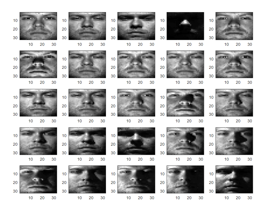
Figure 4. Part of the Yale Extended Face Data data set

The results of applying NMF and PCA to the data are shown in Figures 5 and 6, respectively.

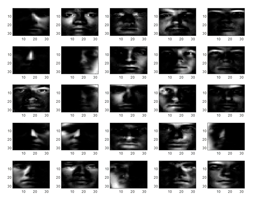
Figure 5. 25 feature sets obtained through NMF

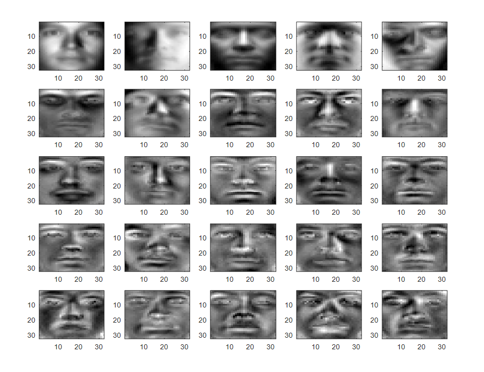
Figure 6. 25 feature sets obtained through PCA

It can be seen that the features obtained through NMF reflect well the direction of light and other structural elements present in the data set. Furthermore, many of the values in NMF features are filled with zeros, indicating that NMF requires less storage space to store features.

Moreover, the features obtained through NMF have a relatively clear meaning compared to those obtained through PCA.

Organizing features by epoch in NMF application results

MATLAB code

The following is MATLAB source code that applies NMF and PCA:

clear; close all; clc;

load('YaleB_32x32.mat'); % gnd seems to be the person number.
% Source: http://www.cad.zju.edu.cn/home/dengcai/Data/FaceData.html
% The name of the used dataset is Extended Yale Face Database B.

figure('position',[556, 237, 947, 699]);
for i= 1:25
    subplot(5,5,i)
    imagesc(reshape(fea(i,:), 32, 32)); colormap('gray')
end

%% Perform NMF
% n_features = 25;
% [W, H] = nnmf(fea, n_features); %using MATLAB function

% Implementing it manually
m = size(fea,1);
n = size(fea,2);
p = 25; % the number of features
rng(1)
W = rand(m, p)*255;
H = rand(p, n)*255;
n_epoch = 200;
X = fea;
for i_epoch = 1:n_epoch
    H = H.*((W'*X)./(W'*W*H));
    W = W.*((X*H')./(W*(H*H')));
end

n_features = p;

figure('position',[556, 237, 947, 699]);
for i_features = 1:n_features
    subplot(5,5,i_features)
    imagesc(reshape(H(i_features,:), 32, 32)); colormap('gray');
end

% figure; imagesc(reshape(randn(1, 25) * H, 32, 32)); colormap('gray')

%% Perform PCA

[coeff, score, latent] = pca(fea);

figure('position',[556, 237, 947, 699]);
for i_features = 1:n_features
    subplot(5,5,i_features)
    imagesc(reshape(coeff(:, i_features), 32, 32)); colormap('gray');
end

References

PREVIOUSSingular Value Decomposition(SVD)

NEXTCorrelation and Inner Product