Formula for Divergence Theorem
| THEOREM 1. Divergence Theorem (2D) |
|---|
| Let a vector field be given as $F(x,y) = P(x,y)\hat{i} + Q(x,y)\hat{j}$, and let the direction of the line integral be counterclockwise with respect to the boundary of the area A. Then the following equation holds: |
The Divergence Theorem states that the total flux of a vector field across a closed path is equal to the net outflow or inflow of the field through the entire area enclosed by the path.
Prerequisites
To understand the Divergence Theorem, it is helpful to have a good understanding of the following topics:
- Divergence of a vector field
- Meaning of double integrals
- Line integrals of vector fields
- Flux of a vector field in 2D
Proof of the Divergence Theorem
※ This proof is taken from the book “Mathematical Methods in the Physical Sciences” by Mary L. Boas.
The proof of the Divergence Theorem starts from the Green’s Theorem, which describes the relationship between line integrals and double integrals. The formula for Green’s Theorem is as follows:
\[\oint_C\vec{F}\cdot d\vec{r} = \iint_A\frac{\partial Q}{\partial x}-\frac{\partial P}{\partial y}dxdy\]Let the vector field $\vec{F}(x,y)$ be given as follows:
\[\vec{F}(x,y) = P(x,y)\hat{i} + Q(x,y)\hat{j}\]Since $P(x,y)$ and $Q(x,y)$ are arbitrary functions, we can adjust them as follows:
\[P(x,y) \Rightarrow -V_y\] \[Q(x,y) \Rightarrow + V_x\]Then the left-hand side of equation (2) becomes:
\[\text{Left-hand side of (2)} \Rightarrow \oint_C\vec{F}\cdot d\vec{r} = \oint_C\left(-V_ydx+V_xdy\right)=\oint_C\vec{V}\cdot \hat{n} ds\](If you do not understand the meaning of $\oint \vec{V}\cdot \hat{n} ds$ in the above equation, it may be helpful to review the topic of Flux of a vector field in 2D.)
Here, $\vec{V} = V_x\hat{i} + V_y\hat{j}$.
And the right-hand side of equation (2) becomes:
$\iint_A \frac{\partial Q}{\partial x} - \frac{\partial P}{\partial y} dxdy = \iint_A \frac{\partial V_x}{\partial x} + \frac{\partial V_y}{\partial y}$.
In fact, the ideas behind Equations (4) and (5) can be traced back to the process of rotating the tangent vector to its normal vector by a -90 degree rotation. To briefly review, if we have a vector $\begin{bmatrix} x \ y \end{bmatrix}$ and rotate it by -90 degrees, we get $\begin{bmatrix} 0 & 1 \ -1 & 0 \end{bmatrix} \begin{bmatrix} x \ y \end{bmatrix} = \begin{bmatrix} y \ -x \end{bmatrix}$. Thus, the core idea of the process is to swap $x$ and $y$ and change the sign of one of them. For a more detailed discussion on this topic, it may be helpful to refer back to the section on calculating the normal vector of a vector field’s flux (2D) in my blog post.
Now, Equations (6) and (7) are equivalent, so if we connect them with a mathematical equation, we can prove the divergence theorem:
\[\Rightarrow \oint_C \vec{V} \cdot \hat{n} ds = \iint_A \frac{\partial V_x}{\partial x} + \frac{\partial V_y}{\partial y}\]The meaning of the divergence theorem (2D)
Consider an arbitrary vector field $\vec{F}$ and a closed path $C$, as shown in Figure 1 below.
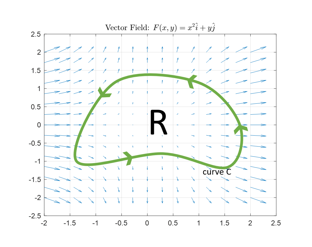
Figure 1. Closed path $C$ and enclosed region $R$ used to explain the meaning of the divergence theorem
As in the case of the Green’s theorem, the explanation for the meaning of the divergence theorem is also based on the fact that the flux result is related to the area integral.
Since the calculation of flux is based on the dot product of vectors, the concept of dot product is the most important one.
First, let’s calculate the flux along the closed path $C$ in Figure 1:
\[\oint_C \vec{F} \cdot \hat{n} ds\]Now, let’s divide the closed path $C$ into two parts as shown in Figure 2 below.
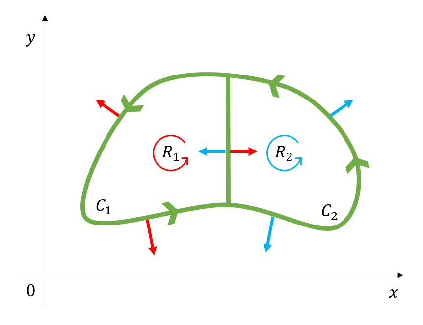
Figure 2. When we divide the closed path C into two paths and calculate the flux for each path, the normal vectors for the two paths can be represented as red and blue arrows, respectively.
In this case, looking at the middle part of the two divided paths in Figure 2, we can see that this path is included in both the $C_1$ and $C_2$ paths simultaneously.
This “simultaneously included path” passes through the same length when calculating the flux for $C_1$ and $C_2$, but since the normal vectors are opposite, the results for calculating the flux for $C_1$ and $C_2$ are the same in magnitude but have opposite signs, so they cancel each other out when added together.
Therefore, if we add the flux values calculated for $C_1$ and $C_2$, we can obtain the flux value for the original closed path $C$. This can be expressed mathematically as follows:
\[\oint_C\vec{F}\cdot\hat{n}ds = \oint_{C_1}\vec{F}\cdot\hat{n}ds+\oint_{C_2}\vec{F}\cdot\hat{n}ds\]Now let’s divide the path we divided in Figure 2 again and divide the original path $C$ into a total of four closed paths, as shown in Figure 3.
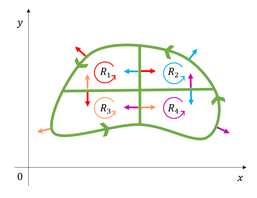
Figure 3. When we divide the closed path C into four paths, the normal vectors for each path can be represented as red, blue, green, and purple arrows, respectively.
Using the same logic as when we calculated the flux values for Figure 2, the flux values for the paths inside the original closed path $C$ all add up to zero when added together. Therefore, the sum of the flux values calculated for all paths $C_1$, $C_2$, $C_3$, and $C_4$ is equal to the flux value for the original path $C$. This can be expressed mathematically as follows:
\[\oint_C\vec{F}\cdot\hat{n}ds = \sum_{k=1}^4\oint_{C_k}\vec{F}\cdot\hat{n}ds\]Using this method, we can also divide the inside of the closed path $C$ into an arbitrary number $N$ of closed paths.
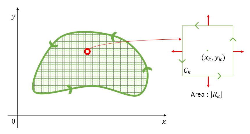
Figure 4. Even if we divide the closed path C into an arbitrary number of paths, when we add up the flux values for the paths inside each divided path, the result will be equal to the flux value for the original path C.
As with the previous discussion, if we calculate the flux values for the $N$ closed paths inside the original closed path and add them together, we will obtain the same flux value as for the original path
\[\oint_C\vec{F}\cdot\hat{n}ds = \sum_{k=1}^N\oint_{C_i}\vec{F}\cdot\hat{n}ds\]Calculation of flux value for the k-th closed path
Let’s consider the k-th closed path $C_k$ as shown in the figure below.
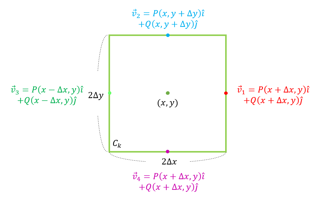
Figure 5. The k-th closed path $C_k$ and vector field at points on the path.
Let the base and height of this path be $2\Delta x$ and $2\Delta y$, respectively, and let the vector values at the four points on the path be denoted as $v_1$ through $v_4$ for the given vector field $\vec{F} = P(x,y)\hat{i}+Q(x,y)\hat{j}$.
\[\vec{v_1} = P(x+\Delta x, y)\hat{i} + Q(x+\Delta x, y)\hat{j}\] \[\vec{v_2} = P(x, y + \Delta y)\hat{i} + Q(x, y + \Delta y)\hat{j}\] \[\vec{v_3} = P(x-\Delta x, y)\hat{i} + Q(x-\Delta x, y)\hat{j}\] \[\vec{v_4} = P(x, y - \Delta y)\hat{i} + Q(x, y - \Delta y)\hat{j}\]One assumption we make here is that $\Delta x$ and $\Delta y$ are small enough so that the vector field does not change along each of the four edges of the closed path $C_k$.
What we ultimately want to calculate is $\oint_{C_k}\vec{F}\cdot\hat{n}ds$, so let’s calculate the integral values for each of the four line segments of the path $C_k$ and add them together.
Let’s calculate them in counterclockwise order from the line segment that vector $\vec{v}_1$ passes through. The normal vector on each line segment has a magnitude of 1 and is in the direction of the $x$ or $y$ axis, so it can be expressed using a unit vector.
\[\text{① }\int_C\vec{v}_1\cdot\hat{n}ds = \vec{v}_1\int_Cds=\vec{v}_1\cdot(\hat{i})2\Delta y\] \[\text{② }\int_C\vec{v}_2\cdot\hat{n}ds = \vec{v}_2\int_Cds=\vec{v}_2\cdot(\hat{j})2\Delta x\] \[\text{③ }\int_C\vec{v}_3\cdot\hat{n}ds = \vec{v}_3\int_Cds=\vec{v}_3\cdot(-\hat{i})2\Delta y\] \[\text{④ }\int_C\vec{v}_4\cdot\hat{n}ds = \vec{v}_4\int_Cds=\vec{v}_4\cdot(-\hat{j})2\Delta x\] \[\text{① + ② + ③ + ④}\Rightarrow \vec{v}_1\cdot(\hat{i})2\Delta y + \vec{v}_2\cdot(\hat{j})2\Delta x + \vec{v}_3\cdot(-\hat{i})2\Delta y + \vec{v}_4\cdot(-\hat{j})2\Delta x\]The meaning of $\vec{v}_1\cdot(\hat{i})$ here is to leave only the $x$ component of $\vec{v}_1$. Therefore, if we expand the equation a bit, we get:
\[\Rightarrow P(x+\Delta x, y)2\Delta y + Q(x, y+\Delta y)2\Delta x - P(x-\Delta x, y)2\Delta y - Q(x, y-\Delta y)2\Delta x\]Combining the terms with $4\Delta x \Delta y$:
\[\Rightarrow 4\Delta x\Delta y\left\lbrace\frac{P(x+\Delta x, y) - P(x-\Delta x, y)}{2\Delta x} + \frac{Q(x, y + \Delta y) - Q(x, y-\Delta y)}{2\Delta y}\right\rbrace\]Here, $4\Delta x \Delta y$ becomes the area $|R_k|$ of the closed path $C_k$, and the value inside the curly braces is similar to the divergence value seen in the article on vector field divergence, but we will call it ‘pseudo-divergence’ here. Let’s use the symbol $pdiv(\cdot)$ to represent pseudo-divergence.
\[\oint_{C_k}\vec{F}\cdot\hat{n}ds\Rightarrow |R_k|pdiv(\vec{F})\]Let’s summarize what we have learned so far.
Therefore, equation (13) can be written as follows:
\[\sum_{k=1}^N\oint_{C_k}\vec{F}\cdot\hat{n}ds = \sum_{k=1}^N|R_k|pdiv(\vec{F})\]If we increase the number $N$ of closed paths $C_k$ we divide the original closed path $C$ into, then $\Delta x$ and $\Delta y$ become very small, and $|R_k|$ can be considered as a small area $dA$, so that pseudo-divergence becomes equivalent to the divergence of the vector field at a single point.
Furthermore, the flux value of the original closed path $C$ is equal to the sum of the flux values of the infinitesimal paths $C_k$ created by dividing it infinitely finely. Therefore, if we make $N$ infinitely large in equation (22), we get:
\[\oint_C\vec{F}\cdot\hat{n}ds = \lim_{N\rightarrow \infty}\sum_{k=1}^N\oint_{C_k}\vec{F}\cdot\hat{n}ds \notag\] \[= \lim_{N\rightarrow \infty}\sum_{k=1}^N|R_k|pdiv(\vec{F})=\iint_A div(\vec{F})dA =\iint_A\left(\frac{\partial P}{\partial x}+\frac{\partial Q}{\partial y}\right)dxdy\]In other words, the divergence theorem states that the flux value of a closed path is equal to the sum of the divergences of small areas obtained by infinitely fine division of the interior of the path.