Until now, we have covered “Signal Representation” while covering Sinusoidal Waves Basics, Complex Number Basics, and Phasor.

From now on, we will learn about the basic properties of systems, linearity and time invariance. A system that has both of these properties is called a Linear Time-Invariant (LTI) system.

Prerequisites

To better understand this posting, it is recommended that you understand the following:

• Signal Processing Introduction
• Sinusoidal Waves Basics
• Phasor

The following knowledge is also good to have but not required to understand the entire content:

• Basic vector operations (scalar multiplication, addition)
• Matrix and Linear Transformation

Any signal can be represented as a combination of sinusoidal waves.

If you were to pinpoint the most critical point of studying signal systems, it would be the statement that “Any signal can be represented as a combination of sinusoidal waves.”

We will study this statement more and more as we go along. It may be difficult to understand right away, but let’s try to become more familiar with it by checking some examples.

Note that it is very difficult to prove this statement mathematically, so it is better to accept it rather than trying to understand it deeply.

In the following picture, we show how a square wave can be represented as a combination of sinusoidal waves.

Figure 1. A square wave represented as a combination of sinusoidal waves
Source: Rala Sun Blog

Signals are not limited to simple square waves, they can also include images. Since an image can also be considered as a signal drawn on a two-dimensional plane, even signals on a two-dimensional plane can be expressed using various periodic waves.

Figure 2. Any signal can be composed of a combination of sinusoidal waves

Then, you might ask, how many combinations of sine waves with different frequencies are needed to express any signal? However, for more details on this topic, please refer to the “Fourier series” or “Fourier transform” section.

The key point I want to make here is that “any signal can be represented as a combination of sine waves.”¹

Now, let’s break down an arbitrary signal into frequency components as shown in the figure below.

Let’s assume that a signal can be distinguished not only by changes over time but also by frequency components.

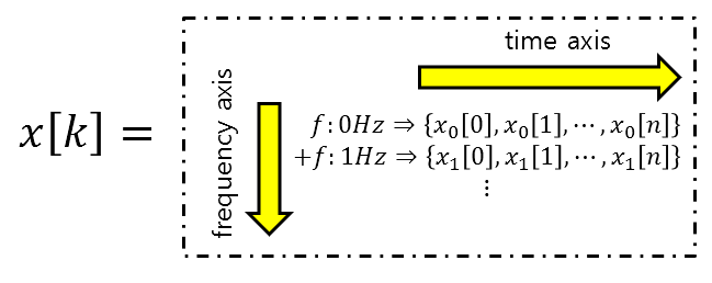
Figure 3. If you think of an arbitrary signal in terms of frequency components, you can break it down into various elements along the time and frequency axes.

You can also think of a signal that you previously thought of as a single horizontal line as actually being composed of a table. The horizontal and vertical axes represent the time and frequency axes, respectively.

In the Introduction to Signal Processing, it was stated that a system is similar to a function that receives an input signal and outputs a transformed signal according to certain “rules.”

And the output signal is transformed from the input signal according to certain “rules.”

If a signal is represented as a table with two axes, frequency and time, it is obvious that if the “rules” are not applied uniformly to certain times or frequency components, the operation will be very complex.

In other words, a simple system should be invariant to changes over time.

Also, it should be possible to apply the same “rules” to each frequency component. In other words, applying the “rules” to each frequency component and combining them should be no different from applying the “rules” to the already combined signal.

Simple is the best. Writing should be simple, rather than difficult, and explaining things simply is more professional than explaining them in a complicated way.

In that sense, we also start studying systems from the simple ones. These “simple” systems are called linear time-invariant (LTI) systems.

Linear Time-Invariant System

Time Invariance

If a system changes as time passes, the system becomes more complex because we have to consider different systems at each time point.

Time invariance can be expressed as follows: if the input is delayed by $n_0$, and the output is also delayed by the same amount, the system is called time-invariant.

\[x[n-n_0] \longmapsto y[n-n_0]\]

To check the time-invariance of a system, we can first apply a delay to the input signal and pass it through the system. Then, we can compare the result with the result obtained by passing the input signal through the system and then applying the delay.

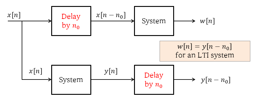
Figure 4. Schematic diagram of a test that can be performed to check time-invariant characteristics

For example, let’s consider the following system:

\[y[n]=(x[n])^2\]

To see if this system is time-invariant, let’s check the following two cases:

\[w[n]=(x[n-n_0])^2\] \[y[n-n_0]=(x[n-n_0])^2\]

Since $w[n]=y[n-n_0]$, this system is time-invariant.

On the other hand, let’s consider the following system:

\[y[n]=x[-n]\]

To check if this system is time-invariant, let’s check the following two cases:

\[w[n]=x[(-n)-n_0]\] \[y[n-n_0]=x[-(n-n_0)]\]

Here, since $w[n]\neq y[n-n_0]$, this system is not a time-invariant system.

Linearity

As previously explained, if the system needs to be applied differently for each component within a signal, the system becomes complicated. Therefore, by using a system that satisfies linearity, the operation of applying the system can be simplified.

Linearity is defined as follows. If $x_1[n]\longmapsto y_1[n]$ and $x_2[n] \longmapsto y_2[n]$, then the following holds true if the system is linear.

\[x[n]=\alpha x_1[n]+\beta x_2[n] \longmapsto y[n]=\alpha y_1[n]+\beta y_2[n]\]

In a linear system, applying the system to each signal component within a signal by multiplying by a constant and adding the results together is possible. (This is also called the principle of superposition.)

Therefore, it is necessary to sufficiently understand the method of dealing with each frequency separately, rather than handling all frequencies at once. (The Phasor method is a way of handling one frequency at a time.)

Also, if we think carefully about the above equation with $\alpha,\beta = 1$, then

\[x[n]=x_1[n]+x_2[n] \longmapsto y[n]=y_1[n]+y_2[n]\]

and by using a single constant,

\[x[n]=\alpha x_1[n] \longmapsto y[n]=\alpha y_1[n]\]

This is the same as writing about basic operations of vectors (scalar multiplication, addition).

Therefore, saying that a system satisfies linearity is the same as saying that a signal can be seen as a vector.

Furthermore, a system that satisfies linearity can be viewed as a linear transformation.

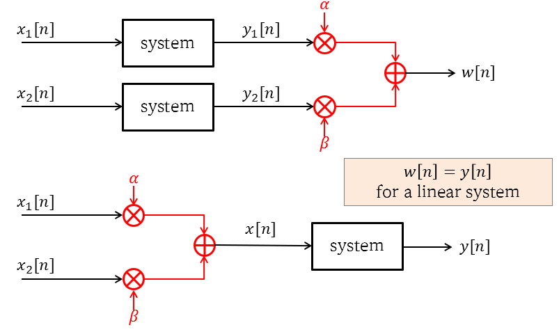
Figure 5. A schematic diagram of a test that can be performed to check linearity.

For an example of determining whether a system is linear, consider the system $y[n]=(x[n])^2$.

To determine whether this system is linear, consider the following two functions:

\[w[n]=\alpha(x_1[n])^2 + \beta (x_2[n])^2\] \[y[n]=(\alpha x_1[n])+\beta (x_2[n])^2 = \alpha^2 (x_1[n])^2 + 2\alpha\beta x_1[n]x_2[n]+\beta ^2 (x_2[n])^2\]

Since it can be seen that these two functions are different, the squared system is a nonlinear system.

Usefulness of LTI Systems

In the end, using linear systems allows signals to be treated like vectors, and systems can be treated as linear transformations.

And using Time-Invariant systems, the same system can be applied for transformation at all time points, making calculations more convenient overall.

This means that the concepts used in linear algebra can be extended to the signal/system field. These concepts form the basis for extending vector space concepts to the signal space.