※ The content of this post is written to provide an easier understanding of the concept of Green’s function rather than mathematical rigor. If there are any fatal errors mathematically, please advise.

Understanding the Solution of Differential Equations using Green’s Function

This post aims to provide an intuitive understanding of the concept of Green’s function, rather than focusing on mathematical rigor. If there are any fatal mathematical errors, please advise.

Prerequisites

To understand the solution of differential equations using Green’s function, it is recommended to have an understanding of the following:

• A Different Perspective on Matrix Multiplication
• Meaning of Row Vectors and Inner Products
• Linear Operators and Function Spaces

Can we think of the Inverse Matrix of a Linear Operator?

In the previous post, Linear Operators and Function Spaces, we learned that we can treat functions as vectors and interpreted differential equations from the perspective of differential operators. We also learned that a linear operator is an extension of the concept of matrices studied in linear algebra, which takes a function as input and outputs another function.

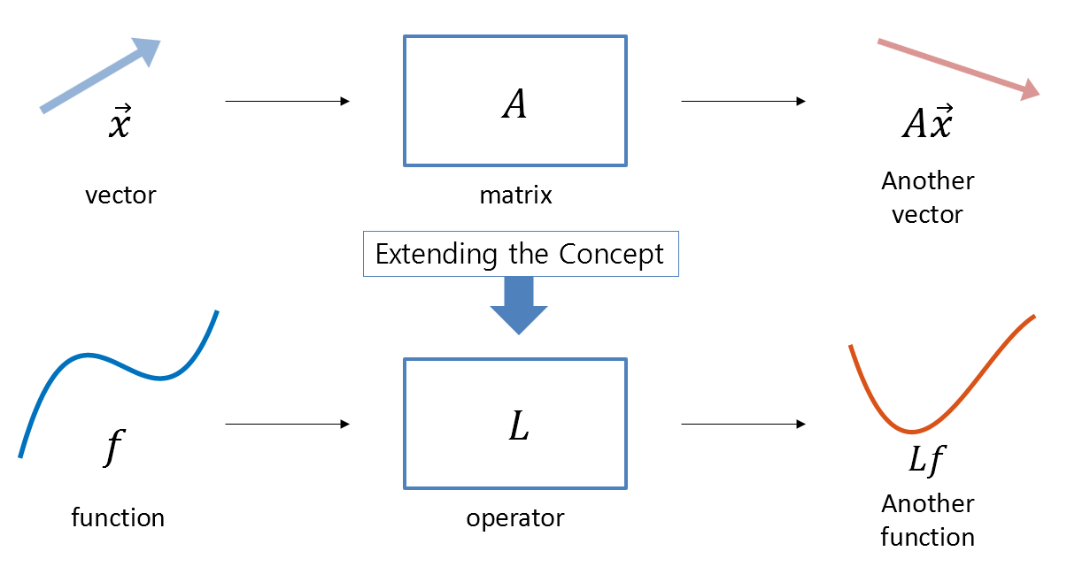
Figure 1. An operator is a function that takes an input function and outputs another function. This concept can be considered as an extension of matrices in linear algebra.

Now, let’s think about the inverse matrix.

The inverse matrix is a matrix defined as follows. Let $A$ be an arbitrary square matrix and $x$ and $b$ be vectors. Assume that the following equation holds:

\[Ax=b\]

If the matrix $A$ has an inverse matrix, $B$, then $B$ satisfies the following property:

\[AB=I\]

Here, $I$ is the identity matrix.

We usually use $A^{-1}$ to denote the inverse matrix, but here we have emphasized that the inverse matrix is also a type of matrix.

As emphasized in operator theory, when extending a concept to another field, one must doubt and doubt again. And one should think several times about the original meaning of the concept to be extended.

Let’s rethink the meaning of matrix multiplication and inverse matrix.

Meaning of Matrix Multiplication and Inverse Matrix

Let’s think again about matrix multiplication.

When we see the equation $AB=I$, we can see the following things happening:

• When the operator $A$ is applied to the first column of $B$, the first unit basis vector is outputted.
• When the operator $A$ is applied to the second column of $B$, the second unit basis vector is outputted.

\[\vdots\notag\]

• When the operator $A$ is applied to the last column of $B$, the last unit basis vector is outputted.

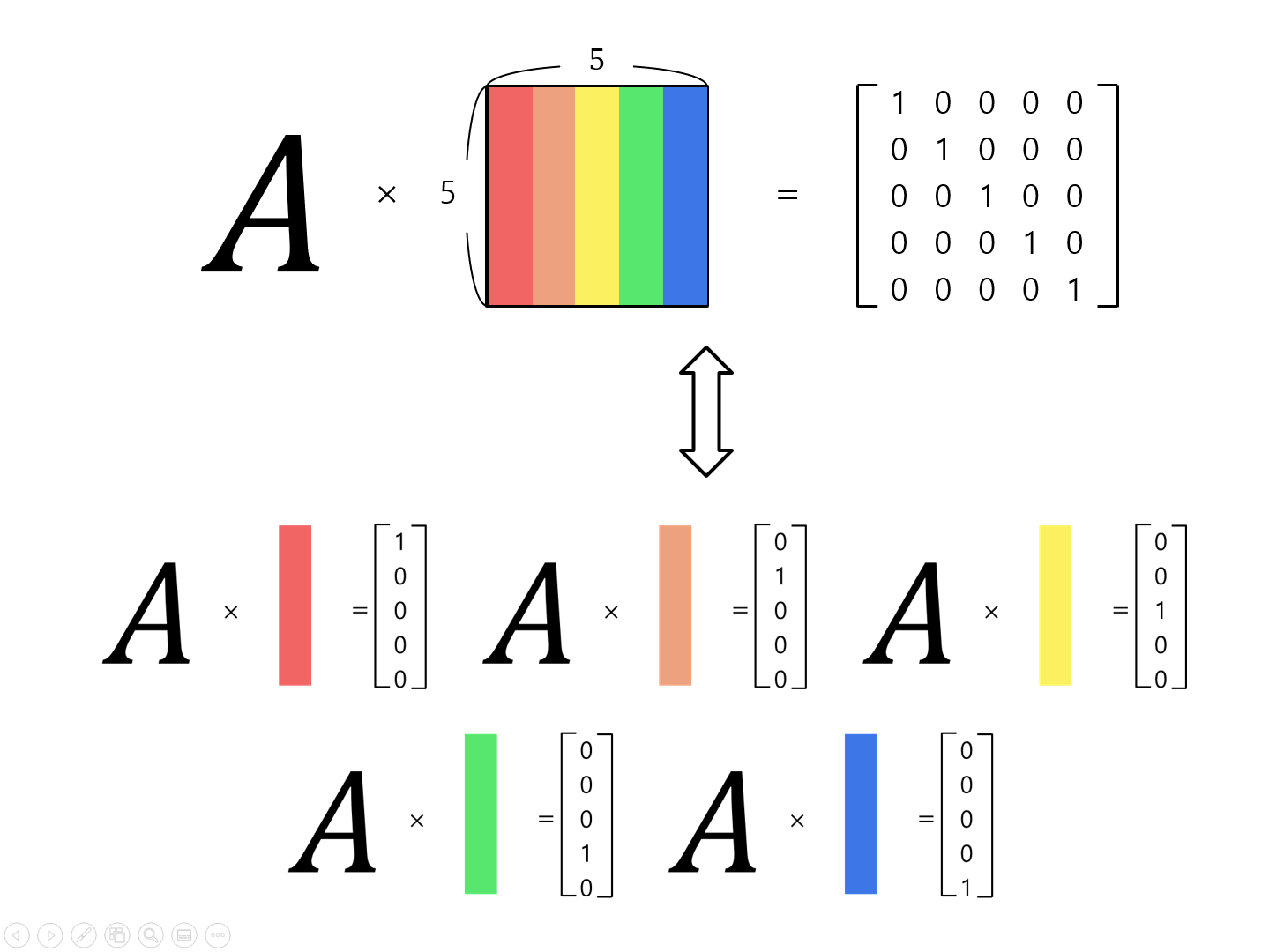
Figure 2. In order for the second matrix to be the inverse of the preceding matrix, which is being multiplied, the preceding matrix must act on each corresponding unit basis vector of the columns of the succeeding matrix.

In Linear Operators and Function Spaces, it was explained that functions can be treated as vectors.

So, if there exists a matrix $B$ such that $AB=I$, the concept corresponding to the matrix $B$ in functional analysis can be seen as something that stacks column vectors, so it can be thought of as something that stacks functions continuously.

In other words, it should be a sequence of functions corresponding to another independent variable rather than the original independent variable.

Let $L$ be a linear operator, and let $u(x)$ and $f(x)$ be functions defined on $x\in[a,b]$. Suppose the following equation holds:

\[Lu=f\]

Let’s represent the ‘sequence of functions’ we will come up with using the following notation:

\[G(x,y)\]

The reason why we wrote a new set of functions with this notation is that $y$ is also a new independent variable defined on the domain $y\in[a,b]$, and we will stack $G(x;y)$ along the new $y$-axis.

Then, if we apply an operator $L$ to follow $y$ on a function $G(x,y)$, we can see that the operation of the inverse matrix performs a similar operation.

• When the operator $L$ is applied to the function corresponding to the first value ($a$) of $y$ in $G(x,y)$, the function corresponding to the first unit basis vector is output.
• When the operator $L$ is applied to the function corresponding to the second value (right next to $a$) of $y$ in $G(x,y)$, the function corresponding to the second unit basis vector is output.

\[\vdots\notag\]

• When the operator $L$ is applied to the function corresponding to the last value ($b$) of $y$ in $G(x,y)$, the function corresponding to the last unit basis vector is output.

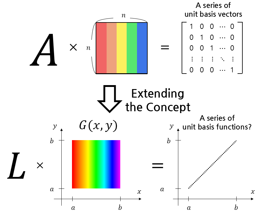
Figure 3. To obtain a function $G(x,y)$ corresponding to the inverse matrix for a certain linear operator $L$, we must be able to output the function corresponding to the unit basis vector when the operator is applied to the function $G(x, y)$ corresponding to each sequence $y$.

Then, we must consider the concept of functions corresponding to unit basis vectors. This concept can be found from the concept of the Dirac delta function.

Unit basis function?

Motivation for Dirac delta function

To think about unit basis vectors, let’s first understand what a unit basis vector is and extend this concept to function spaces.

The simplest unit basis vectors are often called standard bases. In a 2-dimensional vector space, the unit basis vectors are usually called $\hat{i}$ and $\hat{j}$, respectively:

\[\hat{i}=\begin{bmatrix}1\\0\end{bmatrix}\] \[\hat{j}=\begin{bmatrix}0\\1\end{bmatrix}\]

So what is the function of a basis vector? It is to express any arbitrary vector as a linear combination of basis vectors.

For example, any arbitrary vector

\[\begin{bmatrix}a\\b\end{bmatrix}\]

can be expressed as a linear combination of the two basis vectors, $\hat{i}$ and $\hat{j}$, as follows:

\[\begin{bmatrix}a\\b\end{bmatrix} = a\begin{bmatrix}1 \\ 0 \end{bmatrix}+b\begin{bmatrix}0 \\ 1 \end{bmatrix}=a\hat{i}+b\hat{j}\]

Therefore, by taking the dot product of an arbitrary vector with a basis vector, we can obtain the component of the vector that is associated with that basis vector.

For example, for an arbitrary vector $[a,b]^T$, the dot product with the $\hat{i}$ basis vector yields the value $a$:

\[\text{dot}(\begin{bmatrix}a\\b \end{bmatrix}, \begin{bmatrix}1\\0 \end{bmatrix})=a\]

Similarly, we can think of a vector as a list of numbers. Therefore, we can also consider longer lists of numbers.

For example, for a 5-dimensional vector $[2, 3, 5, 1, 4]^T$, by taking the dot product with the basis vector $[1, 0, 0, 0, 0]^T$, we can determine the component of the vector that is associated with that basis vector:

\[\text{dot}\left(\begin{bmatrix}2\\3\\5\\1\\4\end{bmatrix}, \begin{bmatrix}1\\0\\0\\0\\0\end{bmatrix}\right) = 2\]

Similarly, to extract the value of a function at a specific location, we need to consider a function that is similar to a basis vector for taking the dot product.

The dot product of two functions is defined as follows when the interval is properly defined as $[a,b]$:

For functions $f$ and $g$ defined on $x\in[a,b]$,

\[\langle f, g\rangle = \int_{a}^{b}\overline{f(x)}g(x)dx\]

Here, $\overline{f(x)}$ denotes the complex conjugate of $f(x)$.

If $f(x)=\overline{f(x)}$, we can express it as follows:

\[\langle f, g\rangle = \int_{a}^{b}f(x)g(x)dx\]

That is, since the inner product of functions is defined by integration, let’s consider the following function to extract the value of the function using integration:

\[r(x) = \begin{cases}1/(2\epsilon),\quad -\epsilon<x<\epsilon \\ 0,\quad\quad \quad\quad \text{elsewhere}\end{cases}\]

Here, $\epsilon$ is a very small real number.

Since $r(x)=\overline{r(x)}$, we can use the inner product of functions with the following integration:

\[\langle r(x), f(x) \rangle =\int_{a}^{b}r(x)f(x)dx\]

Since the area when integrating this function over the entire domain interval is 1, we can obtain the value of the function $f(x)$ near $f(0)$ by integrating it.

In other words, it means that we can consider the following inner product. If we assume that $x\in[a,b]$ and $a\lt 0\lt b$,

\[\langle r(x), f(x)\rangle=\int_{a}^{b}r(x)f(x)dx\approx f(0)\]

Emergence of Dirac Delta Function

However, the problem is that $r(x)$ is defined only for a suitable width of $2\epsilon$, so it would be difficult to obtain the actual value of $f(0)$ through integration of $f(x)$ and $r(x)$. Therefore, when we make $\epsilon$ very small, we can expect to obtain the value of $f(x)$ more accurately through the inner product in the above equation. When we make $\epsilon$ small, we can see that the following happens:

Figure 4. The shape of $r(x)$ as $\epsilon$ becomes smaller

Therefore, as $\epsilon$ becomes smaller, we can see that $r(x)$ takes the form of $\delta(x)$ below.

\[\delta(x)=\begin{cases}\infty,\quad x=0 \\ 0,\ \ \quad x\neq 0\end{cases}\] \[\int_{-\infty}^{\infty}\delta(x)dx = 1\]

That is, we can obtain the following relation by making $\epsilon$ very small.

\[\int_{a}^{b}\delta(x)f(x)=f(0)\]

Figure 5. By taking the inner product with the Dirac delta function, we can obtain a specific value of the function.

Moreover, if we want to obtain the value of the function at a different position $x_0$ other than $x=0$, we can shift $r(x)$ in parallel and integrate it with $r(x-x_0)$.

Assuming that $x_0$ is located within the interval $[a, b]$,

\[f(x_0) \approx \int_{a}^{b}r(x-x_0)f(x)dx\]

as shown in the above equation.

Here, if we make $\epsilon$ very small,

\[f(x_0)=\int_{a}^{b}\delta(x-x_0)f(x)dx\]

then we can obtain the value of the element of $f(x)$ corresponding to the input of $x_0$.

Figure 6. If we want to obtain the value of the function at an arbitrary position other than $x=0$, we can move the Dirac delta function and perform the calculation.

Ultimately, the Dirac delta function can be considered as a function corresponding to a unit basis vector ¹.

The inverse of the differential operator = Green’s function

Definition of Green’s function

Now that we know that the concept of basis vectors that we were previously considering can be extended through the Dirac delta function, we can properly define the function $G(x,y)$ corresponding to the inverse matrix. This function, which corresponds to the inverse matrix, is called the Green’s function, and its definition is as follows.

Let us assume that the following holds for a linear operator $L$ defined on the interval $x\in[a,b]$ and for functions $u$ and $f$ satisfying appropriate boundary conditions:

\[Lu=f\]

The boundary conditions can be as follows²:

\[u(a)=0, u(b)=0\]

In this case, the Green’s function $G(x, y)$ satisfies the following condition.

\[LG= \delta(x-y)\]

Here, $\delta(x)$ is the Dirac delta function, and $y$ is also a variable defined as $y\in[a,b]$.

Looking at the above equation, we can see that it is similar to the form of

\[AB=I\]

Therefore, we can roughly write

\[G(x,y) \approx L^{-1}\]

To confirm that $G(x,y)$ can be the inverse of $L$, let us multiply both sides of the above equation by $f(y)$ and integrate over $y$.

\[\Rightarrow \int_{a}^{b} L G(x, y)f(y)dy\]

By the definition of the Green’s function, we can rewrite the above equation as follows.

\[\Rightarrow \int_{a}^{b} \delta(x-y)f(y)dy\]

Using the sifting property of the Dirac delta function, we can see that the following holds.

\[\int_{a}^{b}\delta(x-y)f(y)dy = f(x)=Lu\]

On the other hand, since $L$ is a linear operator acting only on $x$, it can also be taken out of the integral.

\[\Rightarrow L\left(\int_{a}^{b} G(x, y)f(y)dy\right)=Lu\]

Therefore, we can find the solution of a differential equation as follows:

\[u(x)=\int_{a}^{b} G(x,y)f(y)dy\]

In other words, the method of finding a solution using the Green’s function is similar to the method of using inverse matrices in linear algebra.

For example, just as the solution of the problem $Ax=b$ can be expressed as $x=A^{-1}b$, the solution of the functional analysis problem $Lu=f$ can be expressed as $u=L^{-1}f$, which can be represented as the integral of the product of $G$ and $f$, similar to the way in which the inverse operation of differentiation is integration.

Example Problem 1

The concept of Green’s functions can be somewhat difficult to understand in practice, even if it is somewhat clear in theory. To supplement this understanding, let’s try solving an example problem using the Green’s function and thinking a bit more about its meaning.

Let’s use the Green’s function to solve the following differential equation:

\[\frac{du}{dx}=x\]

Let’s set the initial condition as $u(a)=0$ and assume that the range of $x$ we are interested in is $x\in[a,\infty)$.

Solution to Example Problem 1

If we think of the differential coefficient as an operator, then our differential operator $L$ is as follows:

\[L=\frac{d}{dx}\]

Using the definition of Green’s function, we can consider the following Green’s function:

\[LG(x,y)=\delta(x-y)\]

First, according to the properties of the Dirac delta function, we can assume the following form of the Green’s function:

\[\begin{cases}LG(x,y) = 0 & \text{for }x\lt y \\ LG(x,y)=0 & \text{for }x\gt y\end{cases}\]

That is, $G(x,y)$ can be expressed as the homogeneous solution of the differential operator $L$ in the intervals where $x\lt y$ and $x\gt y$. In the case where the derivative becomes 0 once, it corresponds to a constant function. In other words,

\[\begin{cases}G(x,y) = c_1 & \text{for }x\lt y \\ G(x,y)=c_2 & \text{for }x \gt y\end{cases}\]

can be written.

On the other hand, if we consider the definition of the Green’s function, we can also think about the following fact.

\[\frac{\partial }{\partial x}G(x,y)=\delta(x-y)\]

(Here, the differential operator $d/dx$ is replaced by $\partial/\partial x$ because $G$ is a function of two variables, $(x, y)$.)

In other words, $G(x, y)$ is a function that has a discontinuous value at the point $x=y$. Moreover, for a sufficiently small positive real number $\epsilon$, we have

\[\int_{y-\epsilon}^{y+\epsilon}LG(x,y)dx=\int_{y-\epsilon}^{y+\epsilon}\frac{\partial}{\partial x}G(x,y)dx\] \[=G(y+\epsilon,y)-G(y-\epsilon,y)=\int_{y-\epsilon}^{y+\epsilon}\delta(x-y)dx=1\]

Therefore, we can imagine that the function has a shape that differs by 1 on both sides with respect to the value of $x=y$.

The rough shape of the Green’s function will be as shown in Figure 7.

When looking at Figure 7, it should be noted that there is a discontinuity when $x$ and $y$ are equal, and the range of $x$ and $y$ is not important. Also, it should be noted that the difference in the function value at the point of discontinuity is 1.

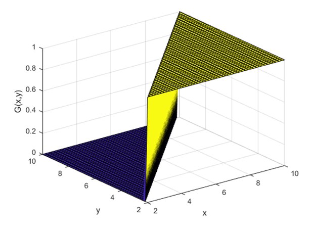
Figure 7. Rough shape of the Green's function when the operator $L$ is a first-order differential operator

Using the initial value condition, we have

\[G(a,y)=0\]

Therefore, we can see from equation (35) that $c_1=0$ and $c_2=1$. Hence,

\[G(x,y) = \begin{cases}0 & x\in [a,y) \\ 1 & x \in (y,\infty)\end{cases}\]

and we can calculate the Green’s function in this way.

This function can also be viewed as the unit step function $H(x)$ shifted positively by $y$.

Here, $H(x)$ has the following form.

\[H(x)=\begin{cases}1, & x\gt 0\\ 0, & x \lt 0\end{cases}\]

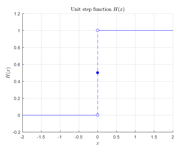
Figure 8. Shape of the unit step function

Therefore, the solution to the differential equation is

\[u(x)=\int_{a}^{\infty}G(x,y)f(y)dy\]

and using the unit step function $H(x)$, we can write it as

\[\Rightarrow \int_{a}^{\infty}H(x-y)f(y)dy\]

where $H(x-y)$ can be understood as a unit step function flipped left and right from the perspective of $y$ and shifted by $x$ to the positive direction.

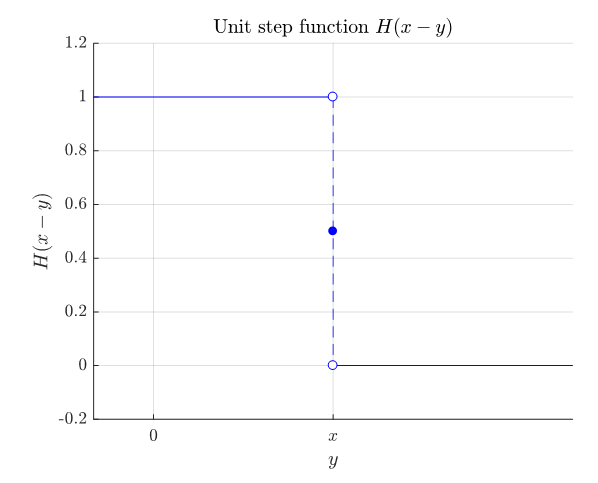
Figure 9. Shape of the unit step function $H(x-y)$

Therefore, we can obtain the solution:

\[u(x)=\int_{a}^{x}ydy=\left[\frac{1}{2}y^2\right]_{a}^{x}=\frac{1}{2}x^2-\frac{1}{2}a^2\]

for the given problem.

Example problem 2

Let’s solve a differential equation involving the second order differential coefficient using the Green’s function.

For instance, consider the following differential equation:

\[\frac{d^2}{dx^2}u=f(x)\]

Assume that the boundary conditions are given as follows:

\[u(0)=0, u(\pi)=0\]

Solution for example problem 2

The given operator $L$ is

\[L=\frac{d^2}{dx^2}\]

Therefore, according to the definition of the Green’s function, we can define the Green’s function as follows:

\[\frac{\partial^2}{\partial x^2}G(x,y)=\delta(x-y)\]

Similar to example problem 1, we need to satisfy the following properties by considering the properties of the Dirac delta function:

\[\begin{cases}LG=0 & \text{for }x\lt y \\ LG=0 & \text{for }x\gt y\end{cases}\]

Thus, we can express $G(x,y)$ as a solution of the homogeneous differential equation of the operator $L$ for the interval where $x\lt y$ and $x\gt y$.

To obtain the second derivative of 0,

\[G(x,y)=\begin{cases} c_1x+c_2 & x\lt y\\c_3x+c_4 & x\gt y\end{cases}\]

should be satisfied. Considering the boundary conditions, we can conclude that:

\[G(0)=c_2=0\]

and

\[G(\pi)=c_3\pi+c_4=0\]

Also, for a sufficiently small positive real number $\epsilon$,

\[\int_{y-\epsilon}^{y+\epsilon}LGdx=\int_{y-\epsilon}^{y+\epsilon}\delta(x-y)dx=1\] \[\Rightarrow \int_{y-\epsilon}^{y+\epsilon}\frac{\partial^2}{\partial x^2}G(x,y)dx=\left[\frac{\partial}{\partial x}G(x,y)\right]_{y-\epsilon}^{y+\epsilon}=1\]

We can see that the second-order partial derivative of $G(x,y)$ at $y=x$ differs by 1, in other words.

Also,

\[G(y+\epsilon,y)-G(y-\epsilon,y)=0\]

In other words, $G(x,y)$ is continuous near $y=x$.

The reason for this can be explained using proof by contradiction. If $G(x,y)$ were discontinuous near $y=x$, then it could be modeled by a unit step function near $y=x$. However, the first derivative of the unit step function is a delta function and the second derivative is a unit doublet function. Therefore, based on the fact that the second derivative of $G(x,y)$ is a Dirac delta function, we can conclude that $G(x,y)$ must be continuous near $y=x$.

Therefore, if we substitute the above conditions,

\[G(y+\epsilon,y)-G(y-\epsilon,y)=c_3y+c_4-c_1y=(c_3-c_1)y+c_4=0\]

and,

\[G'(y+\epsilon,y)-G'(y-\epsilon,y)=c_3-c_1=1\]

We can find the Green’s function as follows.

\[G(x,y)=\begin{cases}\left(\dfrac{y}{\pi}-1\right)x, & x\lt y \\\\ \left(\dfrac{x}{\pi}-1\right)y, & x \gt y\end{cases}\]

If we draw the Green’s function for $y=\pi/3$, we can see that it takes the following form.

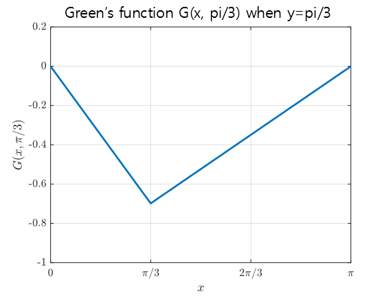
Figure 10. The Green's function for $y=\pi/3$ in Example Problem 2.

The original differential equation $u_{xx}=f(x)$ is a differential equation for the form of waves, and considering that $u(0)=0$, $u(\pi)=0$, it can be said to show a model related to the movement of a rope with both ends fixed.

Also, what the shape of the Green function, as shown in Figure 10, tells us is how the rope is deformed when a force is applied at the point $y=\pi/3$.

The reason why this kind of explanation is possible is that, as seen in the article about the meaning of non-homogeneous differential equations, non-homogeneous terms (in this case, $\delta(x-y)$) are external forcing terms that are unrelated to the autonomous system of differential equations itself.

In other words, $\delta(x-y)$ is an input that is close to an external shock when $x=y$. Therefore, what Figure 10 is referring to is that if an external shock is applied at the position $y=\pi/3$, the state of the rope at that time can be interpreted as being the same as in Figure 10.

(By the way, in signal/system subjects, interpreting the Green function in this way is also called impulse response. Of course, the Time Invariant property must be added. In other words, impulse response can also be seen as a special case of the Green function.)

If $f(x)=x$, the solution can also be obtained as follows.

\[u(x)=\int_{0}^{\pi}f(y)G(x,y)dy=\int_{0}^{x}\left(\frac{x}{\pi}-1\right)y\cdot y ~dy+\int_{x}^{\pi}\left(\frac{y}{\pi}-1\right)x\cdot y~dy\] \[=\frac{1}{6}x^3-\frac{\pi^2}{6}x\]

Example Problem 3

Let’s consider a slightly more complicated form of a second-order differential equation:

\[\frac{d^2}{dx^2}u+k^2u=f(x)\]

Let’s think about the boundary conditions as follows:

\[u'(0)=0, u'(l)=0\]

Solution for Example Problem 3

Similar to the solution for Example Problem 2, we can solve this problem by dividing it into cases where $x<y$ and $x>y$.

For the case where $x<y$, the differential operator $L$ is given by:

\[L=\frac{d^2}{dx^2}+k^2\]

Therefore, the Green’s function for this case is:

\[\frac{\partial^2}{\partial x^2}G(x,y)+kG(x,y)=0\]

So, the Green’s function is:

\[G=A\cos kx+B\sin kx\]

If we substitute the first boundary condition, we get:

\[G=A\cos kx\]

For the case where $x>y$, we can use the same differential operator but substitute the second boundary condition, which gives:

\[G=B\cos k(x-l)\]

The Green’s function that satisfies the continuity condition and the difference of the derivative at $x=y$ being 1 is:

\[G(x,y)=\begin{cases} \cos(kx)\cos(k(y-l))/(k\sin(kl)) & x \lt y \\ \cos(k(x-l))\cos(ky)/(k \sin(kl)) & x \gt y \end{cases}\]

If we assume that $k=1$ and $l=1$, the form of the Green’s function is as follows:

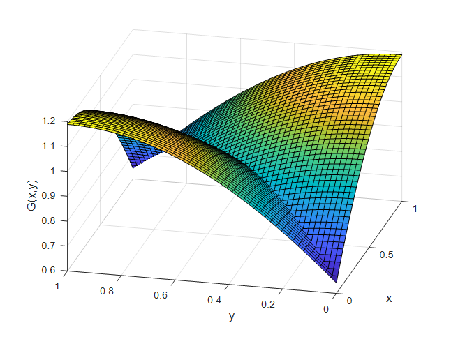
Figure 11. Green's function for Example Problem 3

Using the Green’s function and the function $f(x)$, we can find the solution $u(x)$ by integrating.

References

• Advanced Differential Equations: Asymptotics & Perturbations, J. Nathan Kutz, University of Washington
• Green’s function, Wolfram Alpha
• StackExchange: Green function Impulse response confusion
• Brilliant: Green’s Functions in Physics
• Green’s functions for ODEs, David Skinner, University of Cambridge
• Wikipedia: Green function