Partial Derivatives

Now we are going into multivariate calculus.

So far, we have been taking derivatives of functions with one independent variable and one dependent variable. However, in multivariate calculus, there can be multiple independent variables and multiple dependent variables.

First, let’s look at the simplest form of a multivariate function, where there are two independent variables and one dependent variable.

As an easy example, we can consider the following function:

\[f(x,y) = x^2+xy+y^2\]

If we plot this function using MATLAB, we can draw it as follows:

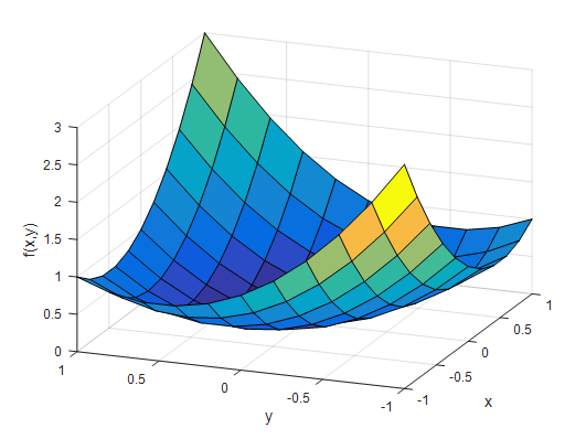
Figure 1. Plot of f(x,y) = x^2 + xy + y^2

In the context of functions, the concept of derivative represents the slope.

However, can we directly calculate the slope of this function using the gradient that we have known so far? If we try to pick an arbitrary point, we can see that the slope line at that point is not uniquely determined.

The concept of partial derivatives arises from the need to calculate the slope in only two perpendicular directions in such situations.

In other words, we want to calculate the slope in the $x$ direction and the slope in the $y$ direction separately by treating $y$ or $x$ as constants and taking derivatives.

Symbolically, the partial derivative of function $f$ with respect to $x$ can be written as:

$f_x$ or $\frac{\partial f}{\partial x}$

Similarly, for $y$:

$f_y$ or $\frac{\partial f}{\partial y}$

represents the partial derivative of the function $f$ with respect to $y$.

Gradient

The gradient outputs a vector that consists of the partial derivative values of $f$ with respect to $x$ and $y$.

It may sound a bit complicated, but it is easy to understand when expressed in the following mathematical notation:

\[gradient(f) = f_x\hat{i}+f_y\hat{j} = \frac{\partial}{\partial x}f(x,y)\hat{i} + \frac{\partial}{\partial y}f(x,y) \hat{j}\]

The above expression for $gradient(\cdot)$ can also be written using the Del (or nabla) operator as follows.

It’s just a symbol, so don’t worry too much.

\[\nabla f=f_x\hat{i} + f_y\hat{j} = \frac{\partial}{\partial x}f(x,y) \hat{i} + \frac{\partial}{\partial y}f(x,y)\hat{j}\]

From what we have seen so far, what does the gradient do? It takes a scalar-valued function and produces a vector value as output. In other words, the input is a scalar, but the output is a vector.

Let’s delve a bit deeper and find the expressions for $\frac{\partial}{\partial x}f(x,y)$ and $\frac{\partial}{\partial y}f(x,y)$ on the right-hand side of $\nabla f$.

\[\frac{\partial}{\partial x}f(x,y) = \frac{\partial}{\partial x}(x^2+xy+y^2) = 2x+y\] \[\frac{\partial}{\partial y}f(x,y) = \frac{\partial}{\partial y}(x^2+xy+y^2) = 2y+x\]

Then, we can see that $\nabla f$ is a function of $x$ and $y$, and it generates a vector for every $x, y$ coordinate. In other words, the gradient is an operator that forms a vector field from a scalar function.

Gradient in the Scalar Plane

Let’s use MATLAB to visualize what the gradient looks like.

Since the output of the gradient is a vector, let’s first examine the vector elements in the $x$ direction.

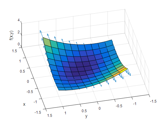
Figure 2. Visualization of the vector components of the gradient in the x-axis direction.

Figure 2 is a top-down view of the same function $f(x, y)$. Each arrow represents only the x-component of the gradient.

As you can see from the figure, only the magnitude in the x-axis direction changes, and each x-component represents the slope in the x-direction.

Let’s now examine the vector elements in the y-direction.

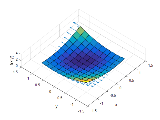
Figure 3. A depiction of the y-axis component of the gradient

Upon careful observation of the figure, you can see that the vectors change only in magnitude in the y-direction at every point in the x, y-plane. The magnitude of each vector represents the slope in the y-direction.

So, what happens if we combine the x-direction and y-direction vector elements together in one graph?

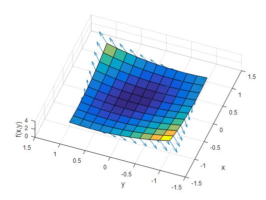
Figure 4. A depiction of the combined vector elements in the x-axis and y-axis components of the gradient

What do the vectors in Figure 4 represent?

They represent the direction of the steepest slope of the $f(x, y)$ plane at each point.

Gradient in a Scalar Field

A scalar field can be represented as $f(x, y, z)$.

A great example of a scalar field is the distribution of temperature. We can think of all the 3D coordinates inside a room and map the temperature corresponding to each coordinate.

For instance, let’s consider that the temperature in 3D space is defined as follows:

\[T(x, y, z) = 20 \times \exp\left(-(x^2 + y^2 + z^2)\right)\]

Then, the gradient of this scalar function $T$ is as follows:

\[\nabla T = T_x\hat{i} + T_y\hat{j} + T_z\hat{k}\] \[=20 \times \exp\left(-(x^2 + y^2 + z^2)\right)(-2x\hat{i} - 2y\hat{j} - 2z\hat{k})\]

So, what does the scalar field $T(x, y, z)$ look like? If we plot it using MATLAB, it would be depicted as follows:

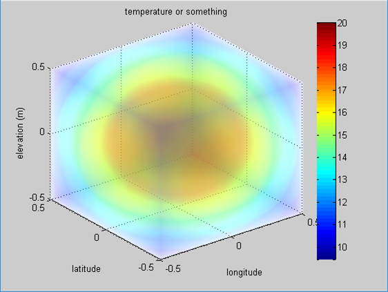
Figure 5. Visualization of the scalar field T for temperature

So, this means that the closer the color is to red, the hotter the temperature is.

Then, what does the gradient mean in this scalar field?

It represents the direction of the greatest change in temperature at any point $(x,y,z)$.

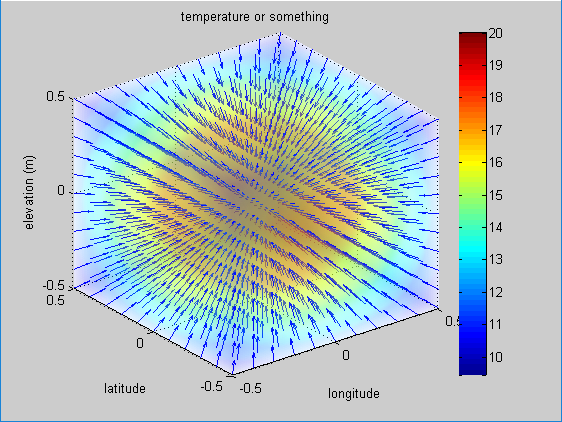
Figure 6. A picture representing the scalar field of temperature T.

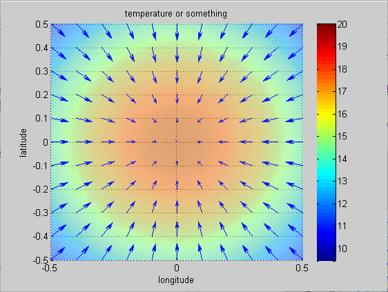
Figure 7. The gradient of Figure 6 viewed from above (view([0 90]).