※ This post is written using the results and source code of the GAN deep learning project in an art museum, available at http://www.yes24.com/Product/Goods/81538614 (in Korean).
※ The source code for this post can be found in Haesun Park’s GitHub repo.
Prerequisites
To understand this post, it is recommended that you have knowledge about the following:
Brief review of AutoEncoder
Variational AutoEncoder (VAE) essentially maintains the form of AutoEncoder (AE).
Therefore, to understand VAE well, it is necessary to understand the characteristics of AE well, to identify the limitations of AE, and to understand what complementary measures VAE has introduced to overcome those limitations.
Let’s briefly review the contents of AutoEncoder.
AE is a neural network that compresses and decompresses data.
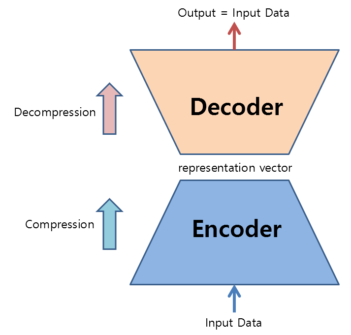
Figure 1. Structure and role of AutoEncoder
To make this possible, when training AutoEncoder, the input of the encoder part and the output of the decoder part should both be the same input data.
The reason for putting in input data and getting the same output data is that we can obtain a slightly lower-dimensional data (representation vector) that can represent the input data nonlinearly.
At this point, the new type of vector obtained by compressing the data is called a ‘representation vector’ or latent factor.
For example, if we use the MNIST dataset, which is a 784-dimensional data (28*28), we can obtain a 2-dimensional representation vector, which can be visualized by attaching labels on a 2-dimensional plane as follows:
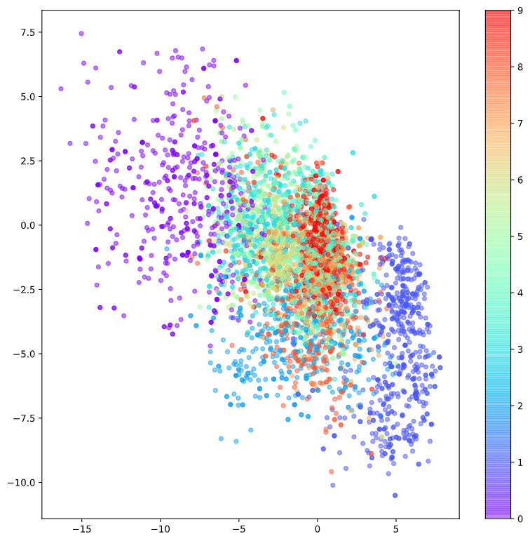
Figure 2. Visualization of the representation vector of MNIST dataset
Through the “compression” process up to this point, the process of transforming high-dimensional data into low-dimensional data is called “encoding,” and the neural network part that performs this task is called the “encoder.”
In addition, an Autoencoder (AE) can also perform “decompression” by selecting arbitrary coordinates in the expression vector space shown in Figure 2 and decoding the data at those coordinates to generate completely new samples that have never been seen before.
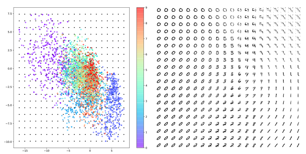
Figure 3. The result of decoding the expression vector obtained through random sampling on the expression vector space
Limitations and Remedies of Autoencoder
So, what are some ways to improve the performance of the Autoencoder (AE), which seems to have implemented the “compression” and “decompression” functions as intended?
First, when generating previously unseen data, the quality of data generated from the empty space in the AE’s latent space is poor. In other words, one could argue that the AE’s decoder function is overfitting to the coordinates where the encoder has encoded specific data.
The second limitation is that the vectors in the expression vector’s vector space are symmetric about (0,0) or have limited values. For example, looking at the distribution of expression vectors in Figure 2, more points are distributed in the negative area of the y-axis than in the positive area. In other words, because there is no specific rule for selecting the location of the expression vectors during encoding, there is a tedious task of always checking where the encoder moved the data in the expression vector space during decoding.
Furthermore, the third limitation is that some numbers are densely packed in a very small area, while others are spread out over a large area. For example, looking at Figure 2, we can see that the number 0 is widely spread in the upper left corner, while the number 9 is densely packed in a very small red area in the center.
So, what is the best way to overcome these three limitations?
Addressing the First Limitation
To address the first limitation, we need to modify the encoder to allow it to place the encoded data points slightly away from their intended positions in the vector space where the encoder would have placed them. This is necessary because the encoder compresses the data and this compression can cause the decoder to overfit the data. One common way to add randomness to the encoder is to use the Gaussian distribution.
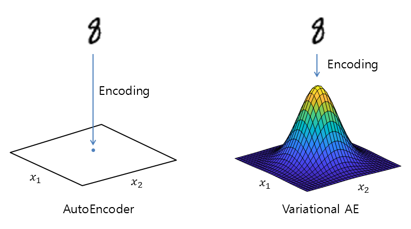
Figure 4. Adding randomness to the encoding coordinates in the vector space can prevent overfitting of the decoder in VAE.
One question that may arise is how to calculate the mean and variance of the Gaussian distribution that will be used to sample the encoding coordinates (i.e., the mean value) for a given input data, such as the ‘8’ shape shown in Figure 4.
In VAE, both the mean and variance values for each Gaussian distribution are calculated as the output values of each fully connected neural network. Of course, the fully connected neural networks responsible for computing the mean and variance values will be trained in the VAE learning process without being aware that the values they are computing are the mean and variance values.
To add randomness to the encoding process, the resulting coordinates are sampled from a normal distribution with mean value equal to the “computed mean” plus “computed standard deviation” times a standard deviation. The resulting point will then be the coordinate where the representation vector is placed.
(Here, the “computed mean” or “computed standard deviation” does not have to be a scalar value. If we consider the vector space of the representation vectors as a two-dimensional vector space, for example, the “computed” mean/standard deviation can be thought of as a two-dimensional vector.)
During the learning process, similar data points (i.e., data points with the same label) will have similar “computed mean” values. Also, the “computed standard deviation” will decrease for all data points as the neural network continues to learn, gaining more confidence in which data points are similar. Ultimately, each label will be clustered as a normal distribution in the vector space.
Addressing the Second Limitation
Regarding the second limitation, we need to impose constraints on the vector space of representation vectors that the encoder embeds. There are various candidate forms, but let’s constrain it to the form of the standard normal distribution, with mean 0 and standard deviation 1.
There is no particular reason why we must do this, but it is to easily sample arbitrary coordinates of the selected representation vector vector space when performing data reconstruction (i.e., decoding) later. In other words, sampling from the standard normal distribution can be easily implemented with a computer.
Let’s use KL divergence as a method of constraining the distribution form, which is a tool that measures how different one probability distribution is from another.
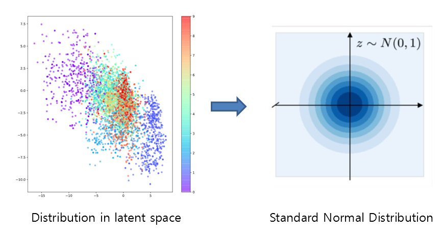
Figure 5. Let's constrain the embedding form in the vector space of representation vectors using KL divergence to the standard normal distribution.
Addressing the Third Limitation
The third limitation can be considered to have already been addressed through the first and second solutions.
Each label must form a cluster while also following the standard normal distribution of the overall embedding distribution. In this process, the encoder will be trained so that the clusters corresponding to each label can be distributed with similar variance as efficiently as possible.
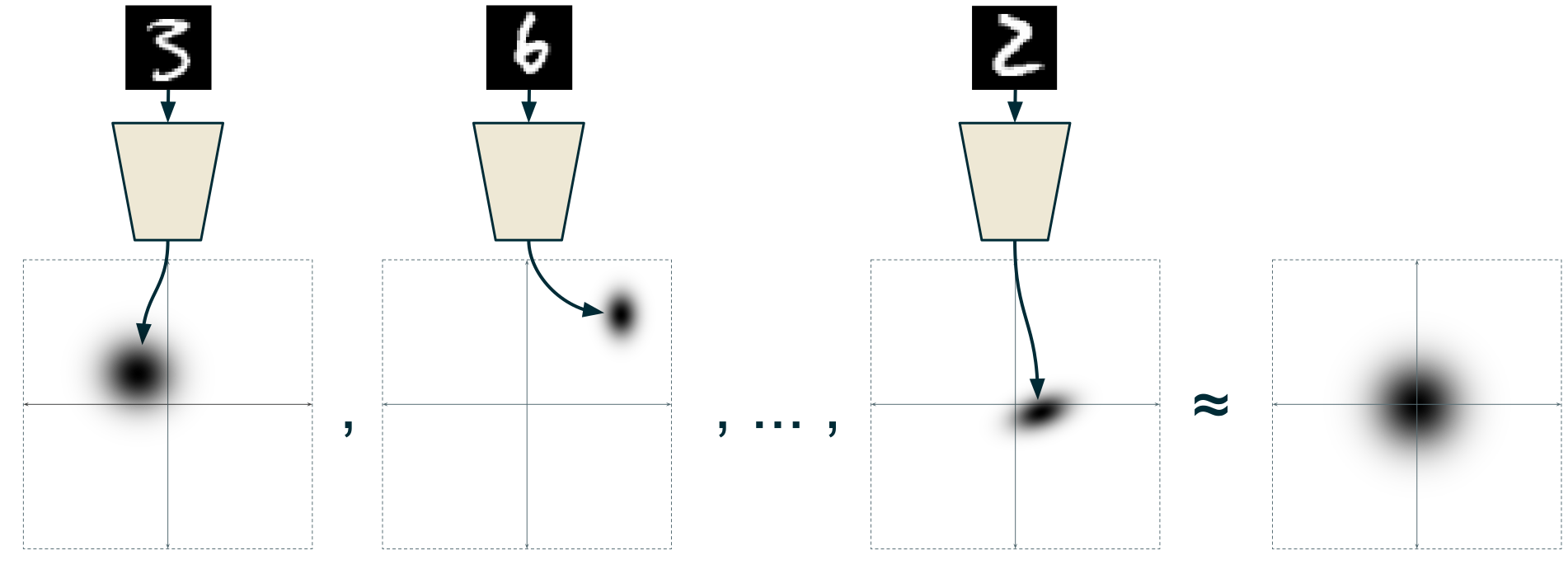
Figure 6. When the shape of each label's cluster and the overall distribution is fixed, the third limitation is naturally resolved.
Figure source: [Isaac Dykeman's blog](https://ijdykeman.github.io/ml/2016/12/21/cvae.html)
The Results of Representation Vector Obtained by VAE
In Figure 7 below, we can see the embedding of the representation vector obtained by VAE in the vector space. Compared to Figure 2, it is clear that the representation vector is spread out more uniformly around the center point (0,0), resembling the shape of a normal distribution. We can also confirm that each label is distributed more uniformly compared to AE.
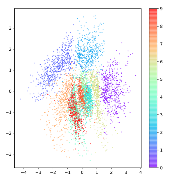
Figure 7. Embedding of representation vector obtained by VAE in the vector space
In addition, in Figure 8, we can see that the reconstructed data obtained by randomly sampling the representation vector in the vector space is more continuous and covers a wider range of numbers compared to the data obtained in Figure 3.
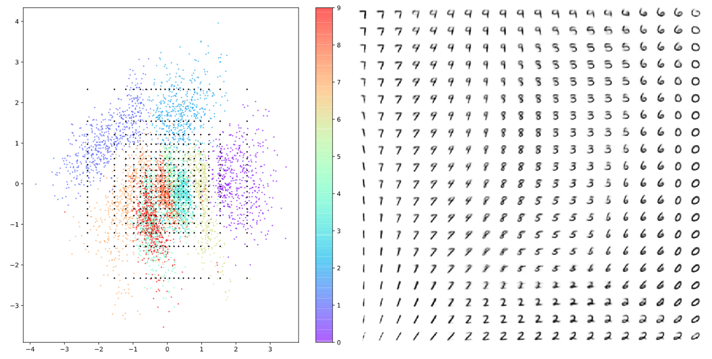
Figure 8. Reconstructed data obtained by randomly sampling the representation vector in the vector space