Prerequisites
To fully understand the content of this post, it is recommended to have knowledge of the following:
Another Perspective on Thinking about ANOVA
When studying ANOVA, the concept of sum of squares is often the biggest hurdle. It may seem like a somewhat unfamiliar concept at first, but the concept of sum of squares is very important in ANOVA. Why do we need to use the sum of squares in the first place?
Usually, when we say “sum of squares” in ANOVA, we actually mean the sum of squares of difference, which is more accurate. When we see this name, two things that we need to think about are: why should we care about deviations, and why should we care about sum of squares?
Firstly, let’s think about deviations. Regardless of what we’re comparing, we need to perform a subtraction (-) to make the comparison possible. That’s not too difficult. It’s a natural logical progression to consider deviations in order to make comparisons.
So why do we square the deviations? Firstly, it is for the purpose of removing sign. Deviations can be positive or negative, making the addition process more complicated. While we can take the absolute value of deviations, taking the square makes the calculation more convenient. That way, we can focus only on the meaning of “variation” regardless of the sign.
However, the reason why sum of squares has survived until now is because the total sum of squares can be thought of as a collection of sum of squares with a special meaning. You may not understand what this means just yet, but if you look at “Understanding ANOVA from the SS perspective” which will be explained later, you may be able to understand it more deeply.
From this point on, let’s abbreviate sum of squares as SS.
Glossary
Before we proceed with understanding ANOVA using SS, let’s review some terms. These may be unfamiliar terms, so I believe referring back to this section repeatedly will be useful for better understanding. Detailed explanations of each term will be added on as we progress through the derivation.
-
If we write $SS_\text{something}$, it means the sum of squares explained by something.
-
Degree of freedom (DF) refers to the number of independent pieces of information that provide information on the population within a given condition when performing statistical estimation using a sample.
If we write $DF_\text{something}$, it means the degree of freedom related to the condition something.
-
Mean square (MS) is the average of SS, which is not an arithmetic average, but rather the value obtained by dividing SS by the degree of freedom.
In other words, it plays a role as a kind of variance in terms of average deviation. However, the reason for distinguishing between variance and mean square is that MS is a statistic that can be modified by degrees of freedom for various reasons.
Understanding One-way ANOVA in terms of SS
In the previous post about the meaning of F-value and ANOVA, we learned about the process of performing ANOVA.
Generally, ANOVA is conducted with the null hypothesis that all sample groups came from the same population.
To check this null hypothesis in ANOVA, two methods are used to estimate variance. The first is to use the variance values that each sample group has, and the second is to estimate variance using the degree to which the mean values of each sample group are spread. If the variance between sample group means is too large compared to the variance within the group, we called it unlikely that the null hypothesis is true. We can then reject the null hypothesis and say that at least one sample group may have been extracted from a different population.
At this time, the ratio value of the variance is called the F-value. That is, the F-value is expressed in the formula as:
\[F=\frac{s^2_\text{bet}}{s^2_\text{wit}}\]Here,
\[s^2_\text{bet}\]is the variance estimated using the mean values of the groups, and
\[s^2_\text{wit}\]is the variance estimated using the standard error within each group.
Since the probability distribution of the F-value is well-known, we can calculate how relatively large the calculated F-value from the given sample group is, and verify the statistical significance through it.
(If you don’t understand the above explanation, we recommend that you check out the previous post about the meaning of F-value and ANOVA.)
Let’s perform the same calculation we did in the previous post about the meaning of F-value and ANOVA.
However, we will rewrite the calculation formula of ANOVA using SS, so the calculation process will be much more complicated than the previous post. You may wonder if it is necessary to go through such a complicated process to get the same result, but in order to perform ANOVA with more complex conditions, this process may be inevitable.
Let’s think about the given dataset as values arranged in a table as below.
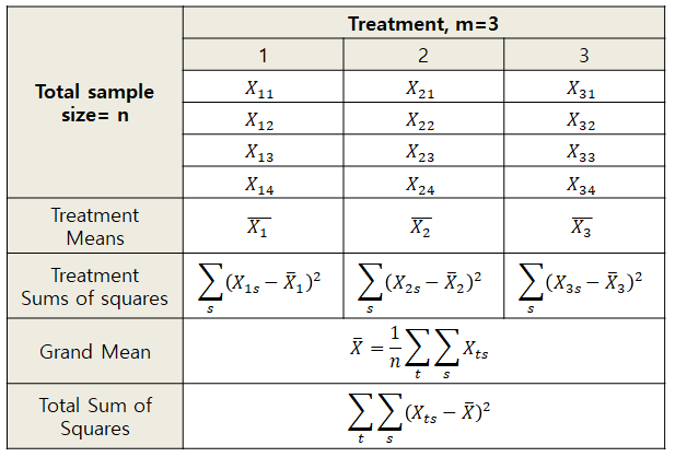
Figure 1. Data used in ANOVA arranged in tables and symbols
Within-group variance ($s^2\text{wit}$) can be calculated by taking the average variance of each treatment group. Specifically, if we denote the variances for each treatment group as $s_1^2, s_2^2, s_3^2$, we can calculate $s^2\text{wit}$ as:
\[s^2_\text{wit}=\frac{1}{3}\left(s_1^2 + s_2^2 + s_3^2\right)\] \[=\frac{1}{3}\left( \frac{\sum_s\left(X_{1s}-\bar{X}_1\right)^2}{n-1} + \frac{\sum_s\left(X_{2s}-\bar{X}_2\right)^2}{n-1} + \frac{\sum_s\left(X_{3s}-\bar{X}_3\right)^2}{n-1} \right)\]Here,
\[SS_1 = \sum_s\left(X_{1s}-\bar{X}_1\right)^2\] \[SS_2 = \sum_s\left(X_{2s}-\bar{X}_2\right)^2\] \[SS_3 = \sum_s\left(X_{3s}-\bar{X}_3\right)^2\]With these notations, we can express $s^2_\text{wit}$ more concisely as:
\[s^2_\text{wit}=\frac{1}{3}\left( \frac{SS_1}{n-1} + \frac{SS_2}{n-1} + \frac{SS_3}{n-1} \right)\] \[=\frac{1}{3}\left( \frac{SS_1+SS_2+SS_3}{n-1} \right)=\frac{\sum_t SS_t}{3(n-1)}=\frac{\sum_t \sum_s\left(X_{ts}-\bar{X}_t\right)^2}{3(n-1)}\]Here, $SS_1+SS_2+SS_3$ represents the sum of squared deviations from the respective treatment means within each group, so let’s write it as $SS_\text{wit}$ instead. Assuming that each group has $n$ samples and there are $m$ groups, we can express the within-group variance as:
\[s^2_\text{wit}=\frac{SS_{wit}}{m(n-1)}=\frac{SS_\text{wit}}{DF_\text{wit}}\]where $DF_\text{wit}=m(n-1)$. Therefore, we know that the within-group variance is equal to $SS_\text{wit}$ divided by $DF_\text{wit}$.
Next, let’s think about between-group variance. Since we know the mean values of each group, we can consider the standard error of each group mean as the standard deviation of the treatment group means.
\[s^2_{\bar{X}}=\frac{s^2_\text{bet}}{n}\]Here $S_{\bar{X}}$ represents the extent to which the means of each treatment are dispersed, that is, the standard error.
Therefore,
\[s^2_{\bar{X}} = \frac{(\bar{X}_1-\bar{X})^2+(\bar{X}_2-\bar{X})^2+(\bar{X}_3-\bar{X})^2}{m-1}\] \[=\frac{\sum_t(\bar{X}_t-\bar{X})^2}{m-1}\]can be found. On the other hand, by slightly adjusting equation (12),
\[s^2_\text{bet}=ns^2_{\bar{X}}\]so,
\[s^2_{\text{bet}}=\frac{n\sum_t(\bar{X}_t-\bar{X})^2}{m-1}\]and it can be seen that the numerator
\[n\sum_t(\bar{X}_t-\bar{X})^2\]refers to the degree by which the average values of each treatment deviate from the grand mean $\bar{X}$. Moreover, we can think about the fact that the degree of freedom when calculating variance from m groups is m-1. Therefore,
\[s^2_{\text{bet}}=\frac{n\sum_t(\bar{X}_t-\bar{X})^2}{m-1}=\frac{SS_\text{bet}}{DF_\text{bet}}\]and we can also express $s^2_{\text{bet}}$ using SS by this formula.
Now, let’s summarize the SS we have learned so far as follows.
\[SS_\text{wit}=\sum_t\sum_s\left(X_{ts}-\bar{X}_t\right)^2\] \[SS_\text{bet}=n\sum_t\left(\bar{X}_t-\bar{X}\right)^2\]Finally, we can think that each sample is the sum of the squared deviations from the grand mean $\bar{X}$, and that is
\[SS_\text{tot}=\sum_t\sum_s\left(X_{ts}-\bar{X}\right)^2\]When we explained the sum of squares (SS), we said that the reason why using the sum of squares survived until the end is because the total sum of squares can be divided into sum of squares with special meanings. As proven below, $SS_\text{tot}$ can be divided into $SS_\text{bet}$ and $SS_\text{wit}$.
\[SS_{\text{tot}}=SS_{\text{bet}} + SS_{\text{wit}}\]Isn’t that it? We can also think of degrees of freedom in the same structure.
\[DF_{\text{tot}}=DF_{\text{bet}} + DF_{\text{wit}}\]
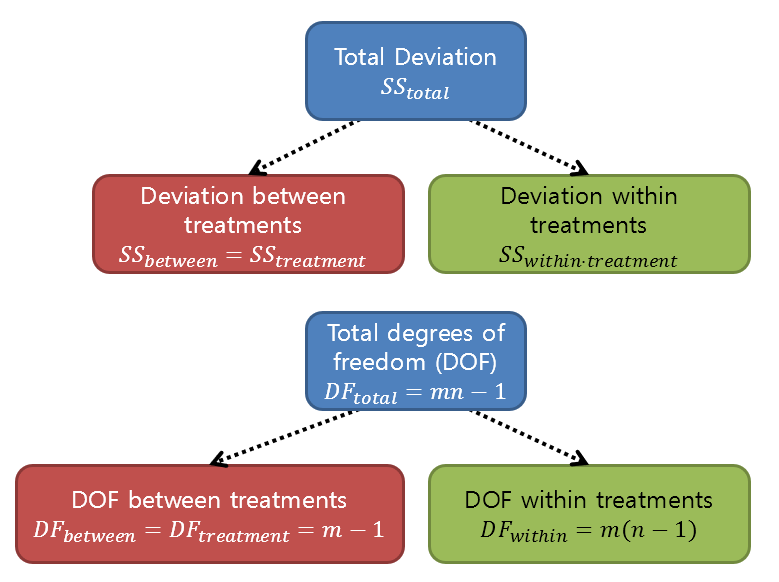
Figure 2. Partitioning of sum of squares and degrees of freedom in one-way ANOVA
By this point, if you were studying ANOVA, you might understand why Sum of Squares (SS) is needed.
SS is studied so that the total SS can be divided into SS with special meanings.
And what it tells us is about the variability caused by a particular meaning, so we can check how much it differs compared to the variability caused by unknown errors.
When calculating the F-value, we don’t use the SS directly but divide the variability expressed as SS by the degrees of freedom to prevent errors that may arise as the number of samples or groups increases.
This time, let’s try to prove that total SS can be divided into between-treatment SS and within-treatment SS mathematically and then solve an example problem.
(Can be skipped) Partitioning of ANOVA Sum of Squares
※ The proof process of $SS_\text{tot}=SS_\text{bet} + SS_\text{wit}$ is not essential. If you find it too complex, you can skip it.
To confirm that $SS_\text{tot}=SS_\text{bet} + SS_\text{wit}$, let’s partition the formula in the parentheses of $SS_\text{tot}$ as follows.
\[(X_{ts}-\bar{X}) = (\bar{X}_t - \bar{X}) + (X_{ts}-\bar{X}_t)\]If we square both sides, we get:
\[(X_{ts}-\bar{X})^2 = (\bar{X}_t - \bar{X})^2 + (X_{ts}-\bar{X}_t)^2 + 2(\bar{X}_t-\bar{X})(X_{ts}-\bar{X}_t)\]Here, if we add up all the samples, we can get the total SS.
\[SS_\text{tot} = \sum_t\sum_s(X_{ts}-\bar{X})^2\] \[=\sum_t\sum_s(\bar{X}_t - \bar{X})^2 + \sum_t\sum_s(X_{ts}-\bar{X}_t)^2 + \sum_t\sum_s2(\bar{X}_t-\bar{X})(X_{ts}-\bar{X}_t)\]The term inside the parentheses of the first term is a term independent of $s$, so
\[\sum_t\sum_s(\bar{X}_t-\bar{X})^2=n\sum_t(\bar{X}_t-\bar{X})^2\]and this is the same as $SS_\text{bet}$.
On the other hand, the third term can be written as follows:
\[\sum_t\sum_s2(\bar{X}_t-\bar{X})(X_{ts}-\bar{X}_t) =2\sum_t\left( (\bar{X}_t-\bar{X})\sum_s(X_{ts}-\bar{X}_t) \right)\]Looking at the innermost formula for $\sum_s$ here,
\[\sum_s(X_{ts}-\bar{X}_t)=\sum_sX_{ts}-\sum_s\bar{X}_t\] \[=\sum_sX_{ts}-n\bar{X}_t\]It could be solved like this, considering the definition of $\bar{X}_t$:
\[\bar{X}_t=\frac{1}{n}\sum_sX_{ts}\]Therefore,
\[\Rightarrow \sum_s(X_{ts}-\bar{X}_t)=\sum_sX_{ts}-n\frac{1}{n}\sum_sX_{ts} = 0\]So,
\[SS_\text{tot} = \sum_t\sum_s(X_{ts}-\bar{X})^2\] \[=\sum_t\sum_s(\bar{X}_t - \bar{X})^2 + \sum_t\sum_s(X_{ts}-\bar{X}_t)^2 + \sum_t\sum_s2(\bar{X}_t-\bar{X})(X_{ts}-\bar{X}_t)\] \[=n\sum_t(\bar{X}_t - \bar{X})^2 + \sum_t\sum_s(X_{ts}-\bar{X}_t)^2 + 0\] \[=SS_\text{bet}+SS_\text{wit}\]is true.
Example problem of One-Way ANOVA
Let’s say we have the following data:
We will test whether at least one of the four groups may have been extracted from a different population.
If we assume that all samples in each group were independently extracted, we can try using One-Way ANOVA.
| Group 1 | Group 2 | Group 3 | Group 4 |
|---|---|---|---|
| 4.6 | 4.6 | 4.3 | 4.3 |
| 4.7 | 5.0 | 4.4 | 4.4 |
| 4.7 | 5.2 | 4.9 | 4.5 |
| 4.9 | 5.2 | 4.9 | 4.9 |
| 5.1 | 5.5 | 5.1 | 4.9 |
| 5.3 | 5.5 | 5.3 | 5.0 |
| 5.4 | 5.6 | 5.6 | 5.6 |
To apply the method previously studied, let’s calculate the within-group variance and the between-group variance using Sum of Squares.
First, let’s calculate the within-group variance $s^2_\text{wit}$.
Calculate the mean for each group and calculate how much it deviates from the mean.
The mean for each group is
\[\bar{X}_1 = 4.9571, \bar{X}_2 = 5.2286, \bar{X}_3 = 4.9286, \bar{X}_4 = 4.8000\]Therefore, for each group, let’s calculate the sum of squares within groups, $SS_1, SS_2, SS_3, SS_4$:
\[SS_1 = (4.6-\bar{X}_1)^2 + (4.7 - \bar{X}_1) ^2 + (4.7 - \bar{X}_1) ^2 + \cdots + (5.4-\bar{X}_1)^2 = 0.5971\] \[SS_2 = (4.6-\bar{X}_2)^2 + (5.0 - \bar{X}_2) ^2 + (5.2 - \bar{X}_2) ^2 + \cdots + (5.6-\bar{X}_2)^2 = 0.7343\] \[SS_3 = (4.3-\bar{X}_3)^2 + (4.4 - \bar{X}_3) ^2 + (4.9 - \bar{X}_3) ^2 + \cdots + (5.6-\bar{X}_3)^2 = 1.2943\] \[SS_4 = (4.3-\bar{X}_4)^2 + (4.4 - \bar{X}_4) ^2 + (4.5 - \bar{X}_4) ^2 + \cdots + (5.6-\bar{X}_4)^2 = 1.2000\]Therefore, $SS_\text{wit}$ is
\[SS_\text{wit}=\sum_t SS_t = 0.5971+0.7343+1.2943+1.2000 = 3.8257\]and $DF_\text{wit}$ is
\[DF_\text{wit} = m(n-1) = 4\times(7-1) = 24\]Therefore, $MS_\text{wit}$ is
\[MS_\text{wit} = \frac{SS_\text{wit}}{DF_\text{wit}}=\frac{3.8257}{24}=0.1594\]Let’s calculate the between-group variance $s^2_\text{bet}$ this time.
Since we’ve already determined the mean for each group, we can calculate the between-group variance by seeing how much each of these means deviate from the grand mean.
The grand mean is
\[\bar{X} = 4.9786\]therefore,
\[SS_\text{bet} = n \sum_{t}(\bar{X}_t-\bar{X})^2\] \[= 7\times \left((4.9571-4.9786)^2+(5.2286-4.9786)^2 +(4.9286-4.9786)^2 + (4.8000-4.9786)^2\right)\notag\] \[=0.6814\]and,
\[DF_\text{bet}=m-1 = 3\]therefore,
\[MS_\text{bet}=\frac{SS_\text{bet}}{DF_\text{bet}}=0.2271\]We can see that the F value we’re trying to find is
\[F = \frac{MS_\text{bet}}{MS_\text{wit}}=\frac{0.2271}{0.1594}=1.4249\]And the p-value of our corresponding F-value is only 0.26 because the numerator and denominator degrees of freedom are both 3 and 24, respectively.
The results of the One-way ANOVA are summarized as follows.
| Source | SS | df | MS | F | Prob > F |
|---|---|---|---|---|---|
| Between | 0.68143 | 3 | 0.22714 | 1.42 | 0.26 |
| Within | 3.82571 | 24 | 0.1594 | ||
| Total | 4.50714 | 27 |
One-Way RM ANOVA
As explained in the Motivation section, Repeated Measures ANOVA (hereafter referred to as RM ANOVA) is a statistical analysis tool that can be applied when a subject undergoes multiple treatments.
While in One-Way ANOVA the total sum of squares (hereafter referred to as SS) is divided into between-group variation ($SS_\text{bet}$) and within-group variation ($SS_\text{wit}$).
In RM ANOVA, on the other hand, the total sum of squares is divided into between-subject variation and within-subject variation, which is further divided into variation caused by treatment and residual variation.
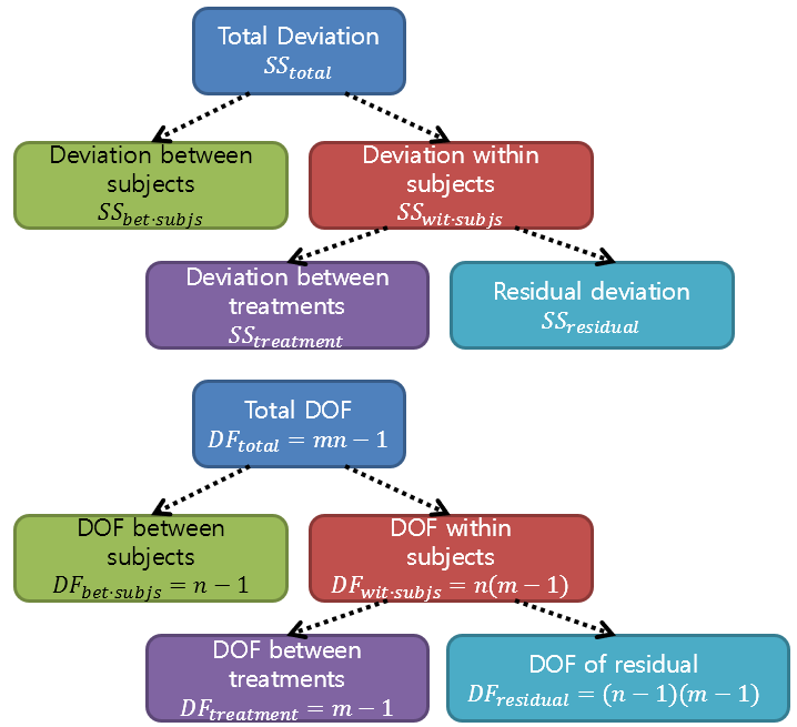
Figure 3. The decomposition of variance and degrees of freedom in repeated measures ANOVA
At first glance, it may seem that the variation is being divided into too many parts, making it difficult to understand, but the most important issue is to accurately capture which variation we are interested in.
If, for example, 100 gym members have their body fat measured three times, what variation should we focus on?
Let’s consider between-subject variation, variation in body fat measurement due to the number of times measured, and residual variation.
Here, we are interested in the variation in body fat measurement over time.
And to statistically handle this, as was done when studying t-tests, we can create an F-value by dividing the variation in body fat measurement over time by the residual variation.
This is because the term “residual variation” implies variation due to errors that cannot be measured.
Therefore, when calculating the F-value, we can divide the variation in body fat measurement over time by the residual variation and then determine its significance.
Calculation Process of RM ANOVA
Let’s take a closer look at the calculation process of RM ANOVA, which we briefly introduced earlier.
First, let’s examine the structure of repeated measures data that can be analyzed using RM ANOVA.
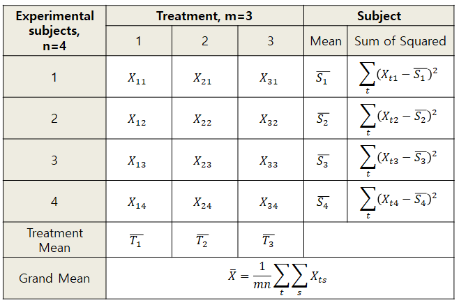
Figure 4. Repeated measures data organized in a table and symbols
In Figure 4, repeated measures data is organized in a table and symbols. At first glance, it may not seem different from the data in Figure 1, but the most significant difference is that the data in Figure 4 refers to the same subject group in each treatment group. For example, in Figure 1, the values in the first row of data ($X_{11}, X_{21}, X_{31}$) are values obtained by different subject participants, but in Figure 4, the values in the first row of data ($X_{11}, X_{21}, X_{31}$) are data obtained by the same subject over three different periods.
Additionally, Figure 4 includes the value of subject mean, $\bar{S}_1, \bar{S}_2, \cdots$, which is calculated as follows:
\[\bar{S}_s=\frac{\sum_t X_{ts}}{m}\]There is also treatment mean value in a similar way, denoted as $\bar{T}_1, \bar{T}_2, \cdots$, which is calculated as follows:
\[\bar{T}_t=\frac{\sum_s X_{ts}}{n}\]Furthermore, there is a grand mean value, $\bar{X}$, which is calculated as follows:
\[\bar{X}=\frac{\sum_t\sum_s X_{ts}}{mn}\]From this, total SS can be calculated as follows:
\[SS_\text{tot}=\sum_t\sum_s\left(X_{ts}-\bar{X}\right)^2\]The freedom degree corresponding to total SS is $mn-1$.
Now, just as total SS could be divided into between-group SS and within-group SS when studying One-Way ANOVA, we can also split total SS in RM ANOVA.
In RM ANOVA, total SS can be divided into within-subject SS and between-subjects SS.
Let’s first take a look at within-subject SS. Within-subject SS is the value that shows how much the reaction value for each treatment that each participant received deviated from the mean value of each participant.
For example, within-subject SS for subject 1 can be calculated as follows:
\[SS_\text{wit subj 1} = \sum_t(X_{t1}-\bar{S}_1)^2\]Similarly, for subject 2, within-subject SS can be calculated in a similar way as follows:
\[SS_\text{wit subj 2} = \sum_t(X_{t2}-\bar{S}_2)^2\]Therefore, within-subject SS for all subjects can be calculated as follows:
\[SS_\text{wit subjs} = SS_\text{wit subj 1}+SS_\text{wit subj 2}+SS_\text{wit subj 3}+SS_\text{wit subj 4}\] \[=\sum_t\sum_s(X_{ts}-\bar{S}_s)^2\]The degrees of freedom for within-subject SS is $m-1$ for each subject, and thus for $n$ subjects it becomes $n(m-1)$.
Next, let’s calculate between-subjects SS. Between-subjects SS represents how far the average values of each subject are from the grand mean, and can be calculated as follows:
\[SS_\text{bet subjs} = m \sum_t(\bar{S}_s-\bar{X})^2\]The multiplication of $m$ is because the average values of each subject represent the average response to $m$ treatments, and this can be seen as the reason for the multiplication.
(This way of thinking is similar to when calculating between-group SS in one-way ANOVA by multiplying the number of groups.)
Since there are $n$ subjects, the degrees of freedom for between-subjects SS becomes $n-1$.
When we have calculated up to this point, we can split the total SS into two necessary SS values as follows:
\[SS_\text{tot} = SS_\text{bet subjs} + SS_\text{wit subjs}\]Finally, let’s divide within-subject SS into SS based on treatment and SS based on residuals.
SS based on treatment can be calculated by using how far each treatment mean is from the grand mean, which gives:
\[SS_\text{treat} = n \sum_t(\bar{T}_t -\bar{X})^2\]The multiplication of $n$ is for the same reason as when calculating between-subjects SS, namely that $\bar{T}_t$ represents an average value which is used to calculate variation using the standard error of the mean.
The degrees of freedom for SS based on treatment is $m-1$.
As mentioned earlier, within-subject SS can be divided into the following:
\[SS_\text{wit subjs} = SS_\text{treat} + SS_\text{res}\]Therefore, we can obtain the residual, which cannot be directly calculated, as follows:
\[SS_\text{res}=SS_\text{wit subjs} - SS_\text{treat}\]The degrees of freedom for the residuals can be calculated as follows:
\[DF_\text{res} = DF_\text{wit subjs} - DF_\text{treat} = n(m-1) - (m-1) = (n-1)(m-1)\]Finally, by using the F value calculated by the variation of the treatment, we can test the null hypothesis that there is no statistically significant difference in treatment at all time points.
\[F = \frac{SS_\text{treat}/DF_\text{treat}} {SS_\text{res}/DF_\text{res}}=\frac{MS_\text{treat}}{MS_\text{res}}\]One of the difficult things when studying RM ANOVA is the terminology of between and within variances that arose when studying one-way ANOVA.
When performing RM ANOVA, the interpretation of all Sum of Squares changes from being about treatment to about subjects.
Refer to the figure below:
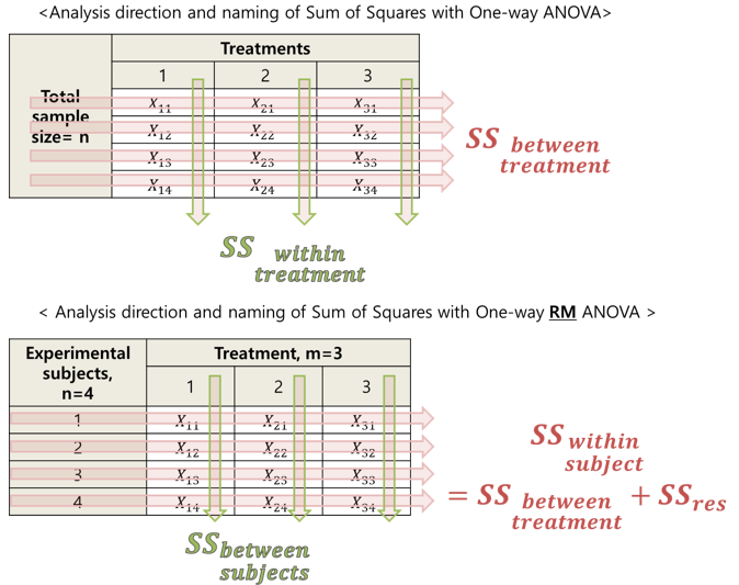
Figure 5. Data structure and SS calculation when using one-way ANOVA and RM ANOVA
When studying one-way ANOVA, the direction of what was vaguely called between variance is horizontal in the upper table of Figure 5. However, when looking at the lower table in Figure 5, the SS calculated horizontally refers to within-subject SS.
When looking at the lower table, we can see that each row represents one subject. Therefore, it can be understood that we calculate Sum of Squares for within subjects, but did you mistakenly think that within-subject refers to within treatment just by seeing the term?
If you had only memorized the terminology of within and between when studying one-way ANOVA, you might have had confusion when studying RM ANOVA. Therefore, I would like to emphasize and caution you to beware of this aspect.
Sphericity
※ For more detailed information on sphericity, please refer to Laerd Statistics’ article. We recommend reading that article for more information.
When conducting RM ANOVA analysis using statistical software, sphericity testing is performed.
Assuming sphericity means that when all treatment differences are combined/compared, it refers to a situation where the variance of all differences is the same.
Looking at the variance of differences is necessary because, during post-hoc analysis, we will perform paired t-tests between time point combinations, and the standard error using the variance of differences will be used as the denominator of the t-value.
Let’s continue talking while looking at the figure below.
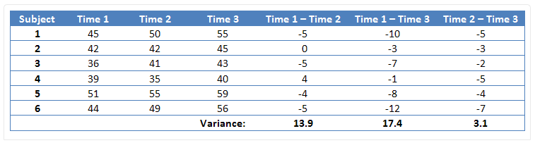
Figure 6. Data where sphericity is not satisfied
Source: Sphericity, Laerd statistics
In the case of Figure 6 above, we checked the data measured three times, calculated the differences between (Time 1 - Time 2), (Time 1 - Time 3), and (Time 2 - Time 3), and compared the variances of these difference values.
Even visually, we can see that the third variance value (3.1) among the three variances (13.9, 17.4, 3.1) is significantly smaller. In such cases, we say that the assumption of sphericity has been violated.
If the assumption of sphericity is violated, the Type I error can increase. That is, there is an increased risk of producing wrong results, indicating that there is a difference when there is actually no difference. The reason for this is that unfair comparisons are made when comparing differences between time points.
Continuing to explain using the case of Figure 6, we can more easily observe significant differences between Time 2 and Time 3 than when comparing Time 1 and Time 2. However, this is not because there was a greater difference between the group means of Time 2 and Time 3, but because the variance of differences between Time 2 and Time 3 was smaller, leading to significant differences being shown.
That is, when performing paired t-tests, the standard error is included in the denominator of the t-value, and this standard error is proportional to the variance of differences.
Therefore, if sphericity is violated when performing RM ANOVA analysis, the Type I error will increase. In fact, even if there is no average difference between time points, a large t-value can be observed between certain time points when the variance of differences is small.
Mauchly’s test
Mauchly’s test is a test that tests sphericity. When conducting RM ANOVA analysis using statistical software such as SPSS, the results of Mauchly’s test are provided.
Mauchly’s W tells us that the closer it is to 1, the more the data satisfies the assumption of sphericity.
Also, the null hypothesis of Mauchly’s test is that the data satisfies the assumption of sphericity. Therefore, if the p-value in the result is greater than 0.05, it can be interpreted that the data satisfies sphericity, and if the p-value is less than 0.05, it can be interpreted that the data does not satisfy sphericity.
Epsilon correction
If the data does not satisfy the assumption of sphericity when performing RM ANOVA, the analysis is conducted by adjusting the degrees of freedom.
That is, if the p-value in Mauchly’s test is less than 0.05, it is determined that the data does not satisfy sphericity, and the degrees of freedom in the result of RM ANOVA can be adjusted by modifying it.
The constant value multiplied to adjust the degrees of freedom is called epsilon. There are two types of epsilon: Greenhouse-Geisser (G-G) epsilon and Huyhn-Feldt (H-F) epsilon.
The epsilon value is a value less than or equal to 1. Therefore, if the data does not satisfy sphericity, the adjustment is made by lowering the degrees of freedom.
This is a reasonable way, as if sphericity is not satisfied, the Type I error rate increases, so decreasing the degrees of freedom makes it easier to not meet the significance level with the same F-value.
To compensate for the increased Type I error rate, the degrees of freedom are lowered in this way.
If you are wondering which to use between G-G epsilon and H-F epsilon, refer to the flow chart below.
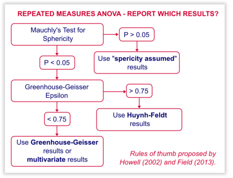
Figure 7. Box plot of data measured over time as shown in Figure 6
Conventionally, when the assumption of sphericity is violated in Mauchly’s test and the G-G epsilon value is less than 0.75, the G-G epsilon is used to adjust the degrees of freedom. On the other hand, if the violation of sphericity is found in Mauchly’s test, but the G-G epsilon value is greater than 0.75, the H-F epsilon value is used to adjust the degrees of freedom.
Example problem of RM ANOVA
Let’s perform RM ANOVA using the data used in Figure 6.
First, if we draw boxplots of the data given in Figure 6 by measurement time, we can see the following.
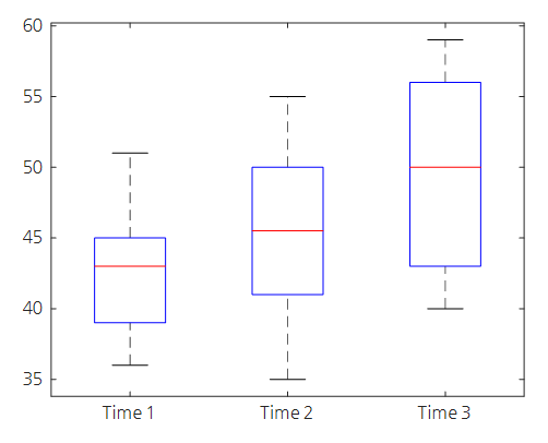
Figure 8. Box plot of data measured over time as shown in Figure 6
Even by visual inspection, we can deduce that the data values tend to increase overall as the measurement time changes.
We need to calculate three types of Sum of Squares: between subject SS, within subject SS, and treatment SS.
To do this, we can calculate the grand mean $\bar{X}$, the mean for each measurement group, and the mean value for each subject as follows 1:
\[\bar{X} = 45.94\] \[\bar{T}=\begin{bmatrix}42.83 & 45.33 & 49.66\end{bmatrix}\] \[\bar{S} = \begin{bmatrix}50.00\\43.00\\40.00\\38.00\\55.00\\49.66\end{bmatrix}\]Looking at the data, we can see that the number of subjects $n=6$ and the number of time points $m=3$.
First, if we calculate between subject SS, we get the following.
\[SS_\text{bet subj}= m \sum_t(\bar{S}_s-\bar{X})^2 = 658.2778\]And the within subject SS is
\[SS_\text{wit subj} = \sum_t\sum_s(X_{ts}-\bar{S}_s)^2 = 200.6667\]Finally, the treatment SS is
\[SS_\text{treat}=n \sum_t(\bar{T}_t -\bar{X})^2 = 143.4444\]And using the difference between within subject SS and treatment SS, we can calculate the residual SS as follows:
\[SS_\text{res}=SS_\text{wit subj} - SS_\text{treat} = 57.2222\]Meanwhile, the degrees of freedom for between subject, within subject, treatment, and residual are as follows:
\[DF_\text{bet subj}=n-1 = 5\] \[DF_\text{wit subj}=n(m-1) = 12\] \[DF_\text{treat}=m-1 = 2\] \[DF_\text{res} = (n-1)(m-1) = 10\]Finally, the interest F value can be calculated as follows:
\[F=\frac{SS_\text{treat}/DF_\text{treat}}{SS_\text{res}/DF_\text{res}}=\frac{MS_\text{treat}}{MS_\text{res}} = 12.5340\]The F value corresponding to p-value = 0.95 with degrees of freedom (2, 10) is:
\[F_{p=0.95}(2,10)=4.1028\]However, since the given F value of 12.5340 is greater than 4.1028, we can conclude that our data shows significant differences in at least one time point.
Jamovi
There are plenty of software that can perform Repeated Measures ANOVA, but if we have to choose a GUI-based software, we would recommend Jamovi.
The reason is that it is free to use. RM ANOVA can be performed on SPSS, Python, and other software as well.
Using Jamovi, you can input the data shown in Figure 6 as follows and perform RM ANOVA.
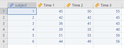
Figure 9. Input data of Figure 6 using Jamovi
Looking at the RM ANOVA analysis results, we can see that we have obtained the same F value as calculated manually earlier.
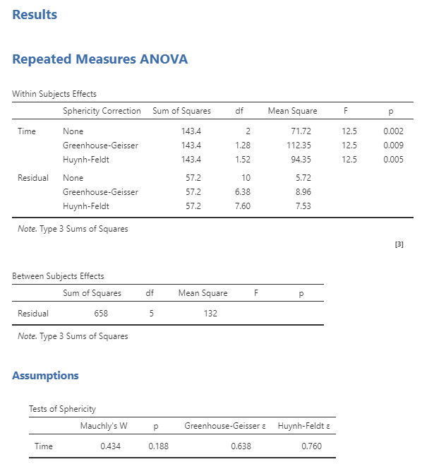
Figure 10. RM ANOVA analysis results obtained using Jamovi
However, it also covers cases where the Mauchly’s test result for sphericity and G-G or H-F epsilon values are applied.
Since it is difficult to calculate sphericity tests and epsilon values manually, it is recommended to use statistical software to do so.
References
- Primer of biostatistics, 7th ed., S. Glantz / Ch. 9 Experiments when each subject receives more than one treatment
- sphericity, Leard statistics
Below is a list of references related to the Jamovi program.
- The jamovi project (2021). jamovi. (Version 1.6) [Computer Software]. Retrieved from https://www.jamovi.org.
- R Core Team (2020). R: A Language and environment for statistical computing. (Version 4.0) [Computer software]. Retrieved from https://cran.r-project.org. (R packages retrieved from MRAN snapshot 2020-08-24).
- Singmann, H. (2018). afex: Analysis of Factorial Experiments. [R package]. Retrieved from https://cran.r-project.org/package=afex.
-
$\bar{T}$ and $\bar{S}$ are row and column vectors, respectively, just following the table format. ↩