이 문서의 한국어 버전은 아래의 위치에서 찾을 수 있습니다. (You can find a Korean version of this article as below.)
Frequency Sampling and DFT
The Purpose of Frequency Sampling
So far, we have learned how to convert an analog signal into a digital signal by sampling it in the time domain and how to reconstruct it back to an analog signal. This concept originates from an everyday idea, which makes it easy to understand why we need the Nyquist Sampling Theorem or the concept of ideal reconstruction.
But why do we need to sample in the frequency domain? It’s because all digital systems are discrete. Analyzing the frequency response of a signal using discrete-time signals or sampling a CT signal may seem possible, like it is in a computer. However, it’s impossible to analyze the frequency response of a DT signal that isn’t a periodic signal. This is clearly shown in the equations defining DTFS and DTFT.
| DEFINITION: Discrete Time Fourier Series (DTFS) |
|---|
| For periodic discrete time signals, where $$a_k=\frac{1}{N}\sum_{n=N_1}^{N_2}x[n] \exp\left(-j\frac{2\pi k}{N}n\right)$$ |
| DEFINITION: Discrete Time Fourier Transform (DTFT) |
|---|
| For discrete time signals, where $$X(f)=\sum_{n=-\infty}^{\infty}x[n]\exp(-j2\pi fn)$$ |
Looking again at the equation for the DTFT, we can see that both $x[n]$ and $X(f)$ have a continuous frequency variable $f$. Therefore, if we want to use a computer to analyze the frequency response of a general discrete-time signal $x[n]$, it is inevitable that we need to sample the continuous frequency variable $f$.
Sampling DTFT
Before we sample continuous frequencies, there are some facts we need to address. Although we call the signal we receive through computers any discrete time signal $x[n]$, its length is always finite. Therefore, let’s define the length of a general discrete signal $x[n]$ to be $N$ for use in computers. Then, the DTFT $X(f)$ can be thought of as follows:
\[\hat{X}(f)=\sum_{n=0}^{N-1}x[n]\exp(-j2\pi fn)\]Now, let’s convert continuous frequency to discrete frequency. If we recall the derivation process of CTFT and DTFT, we can easily see that this can be done because the continuous frequency $f$ started from $\lim_{N\rightarrow\infty}{\frac{k}{N}}$. Therefore,
\[\hat{X}[k] = \sum_{n=0}^{N-1}x[n]\exp\left(-j\frac{2\pi k}{N}n\right)\]Now, we can define the above $\hat{X}[k]$ as a new Fourier transform, the Discrete Fourier Transform.
| DEFINITION: Discrete Fourier Transform (DFT) |
|---|
| For a discrete signal $x[n]$ whose total signal length is N, |
Now, let’s derive the inverse Discrete Fourier Transform. As with Fourier Analysis Series, we can use the property of orthogonality.
PROOF Derivation of inverse DFT
The DFT is defined as follows:
\[X[k] = \sum_{n=0}^{N-1}x[n]\exp\left(-j\frac{2\pi k}{N}n\right)\]Let us consider the following equation for two integers $p$ and $n$ and use the property of orthogonality of discrete signals:
\[\sum_{p=0}^{N-1}X[k] \exp\left(j\frac{2\pi p}{N}k\right)\] \[=\sum_{p=0}^{N-1} \sum_{n=0}^{N-1}x[n]\exp\left(-j\frac{2\pi k}{N}n\right) \exp\left(j\frac{2\pi p}{N}k\right)\] \[=\sum_{p=0}^{N-1}\sum_{n=0}^{N-1}x[n] \exp\left(j\frac{2\pi(p-n)}{N}k\right)\]Here, as in the CTFS, we can consider two cases: $p\neq n$ and $p=n$.
1) In the case where $p\neq n$, we can use the orthogonality property to obtain:
\[Eq (9) = \sum_{p=0}^{N-1}X[k] \exp\left(j\frac{2\pi p}{N}k\right) = 0\]1) In the case where $p=n$, we can use the orthogonality property to obtain:
\[Eq (9) = \sum_{p=0}^{N-1}X[k] \exp\left(j\frac{2\pi p}{N}k\right) = Nx[n]\]Therefore, the inverse DFT is given by:
\[x[n] = \frac{1}{N}\sum_{k=0}^{N-1}X[k] \exp\left(j\frac{2\pi k}{N}n\right)\]| DEFINITION: inverse Discrete Fourier Transform (iDFT) |
|---|
| For a discrete signal $x[n]$ whose total signal length is N, |
Let’s learn more about DFT through an example.
Ex) Find the DFT $X[k]$ of the discrete signal $x[n]$ below.
\[x[n] = \begin{cases} 1, & n = 0, 1, 2, 3 \\ 0, & \text{otherwise} \end{cases}\]Sol)
By definition of DFT,
\[X[k] = \sum_{n=0}^{3} 1 \times \exp\left(-j\frac{2\pi k}{4}n\right)\] \[= 1 + \exp\left(-j\frac{\pi}{2}k\right) + \exp\left(-j\pi k\right) + \exp\left(-j\frac{3\pi}{2}k\right)\]Therefore, when $k=0$, $X[0]=4$. When $k= 1,2,3$, $X[k]=0$.
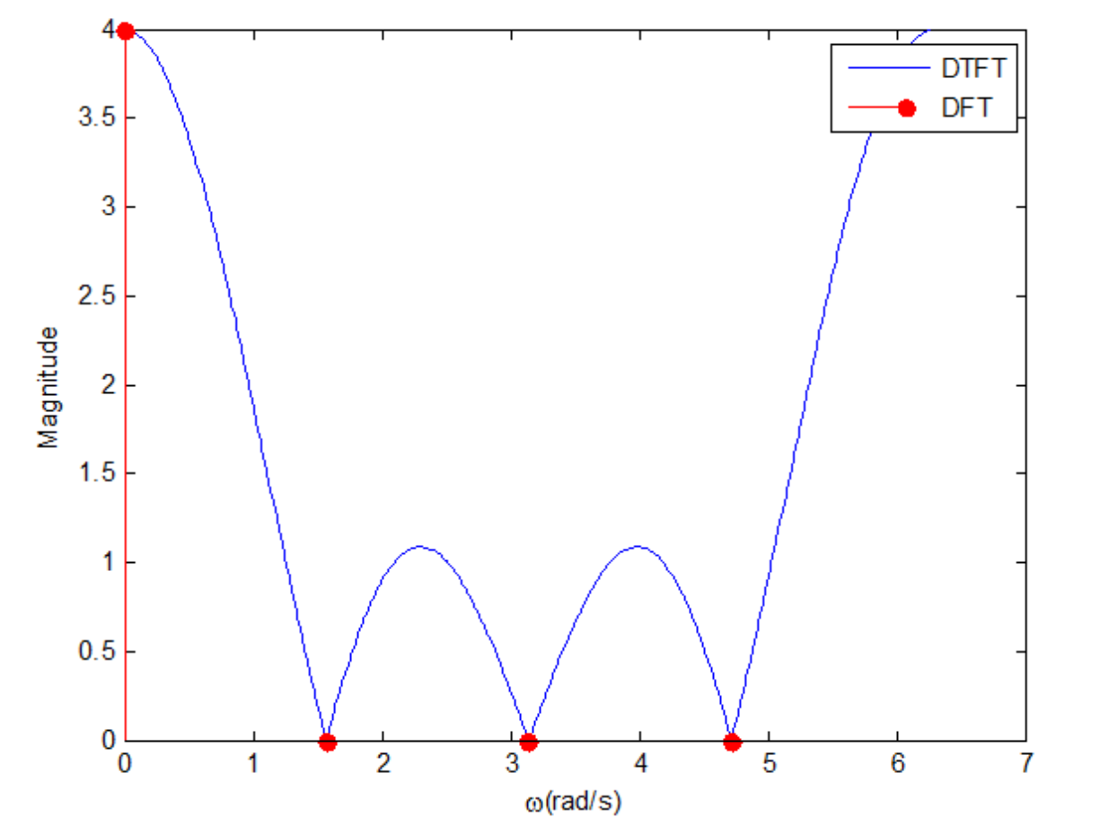
Through solving the simple example above, what can we learn? We can see whether the result of DTFT of $x[n]$ has been properly sampled in the frequency domain. By solving the same problem, we can obtain the DTFT $X(f)$ of $x[n]$ as follows.
ex2) Find the DTFT $X(f)$ of the discrete signal $x[n]$ below.
\[x[n] = \begin{cases} 1, & n = 0, 1, 2, 3 \\ 0, & \text{otherwise} \end{cases}\]Sol)
\[X(f) = \sum_{n=0}^{3}\left(1\times \exp({-j2\pi fn})\right)\] \[=\frac{1-\exp({-j8\pi f})}{1-\exp({-j2\pi f})}\]The equation above can be changed as follows.
\[= \frac {\frac{\exp({j4\pi f})-\exp({-j4\pi f})}{\exp({j4\pi f})}} {\frac{\exp({j\pi f})-\exp({-j\pi f})}{\exp({j\pi f})}}\] \[= \frac{\exp({j\pi f})}{\exp({j 4\pi f})} \times \frac{\exp({j 4\pi f}) - \exp({-j 4\pi f})}{\exp({j \pi f}) - \exp({-j \pi f})}\] \[=\exp\left(-j 3\pi f \right) \frac{\sin(4\pi f)}{\sin(\pi f)}\]By substituting the frequency $f$ in the answer of Ex2 with $\frac{k}{4}$, we can discretize the frequencies. As a result, we can see that we get the same result as in Ex1 for each $k=0,1,2,3$. This discretization of frequencies can be confirmed through the following graph.
Representation of Frequency-Sampled Frequency Response in Time Domain
First, let’s reconsider what happens when we sample time. We have previously proven that when we sample time, we show periodicity in the frequency domain. In other words, since time and frequency have a dual property, a signal sampled in the frequency domain will have periodicity in the time domain.
Let’s denote a signal that is sampled with M samples in the continuous frequency domain $X(f)$ as $X_s[k]$. In other words, $X_s[k]$ can be represented using the discrete frequency $f_k = \frac{k}{M}$ for $k=0,1,\cdots,M-1$. We can mathematically prove this using the technique used for sampling in continuous time domain.
\[X_s[k] = X\left(e^{j\frac{2\pi k}{M}}\right) = X(f) P(f)\]Furthermore, based on the time sampling theory,
\[p[n] = \sum_{l=-\infty}^{\infty}\delta[n-lM]\]Also, since $X_s[k]=X(e^{j\frac{2\pi k}{M}})=X(f)P(f)$, we have $x_s[n]=x[n]\otimes p[n]$.
Therefore \(x_s[n] = x[n] \otimes \sum_{l=-\infty}^{\infty} \delta[n-lM] = \sum_{l=-\infty}^{\infty} x[n]\otimes \delta[n-lM]\)
This implies that:
\[x_s[n] = \sum_{l=-\infty}^{\infty}x[n-lM]\]That is, according to the above result, the inverse DFT $x[n]$ is a periodic function with a period of M. Also, to prevent aliasing of the N-sample discrete signal $x[n]$ represented in the Discrete Time Domain, we need to divide the continuous frequency into M discrete frequencies where $N\leq M$.
Understanding DFT Using Fourier Matrix
Another way to understand DFT is to vectorize the signal and view Fourier transform as a linear transformation through Fourier matrix.
First, let’s look at the definitions of DFT and iDFT.
| DEFINITION: DFT and iDFT |
|---|
| For a discrete signal $X[n]$ of length N and its discrete frequency components $X[k]$ of length N, |
If we think about it, a signal $x[n]$ of length N can be thought of as an N-dimensional column vector, and similarly, its discrete frequency components $X[k]$ of length N can also be thought of as an N-dimensional column vector.
In other words, the signal can be vectorized as
\[\begin{bmatrix}x[0]\\ x[1] \\ \vdots \\ x[n] \\ \vdots \\ x[N-1]\end{bmatrix}\]and the corresponding frequency components obtained through appropriate linear transformation are
\[\begin{bmatrix}X[0]\\ X[1] \\ \vdots \\ X[k] \\ \vdots \\ X[N-1]\end{bmatrix}\]We can think of the frequency components obtained through the signal vector using a matrix (in this case, the Fourier matrix). To understand this, let’s calculate the value of $X[k]$ for $k=0,1,\cdots, N-1$ one by one.
\[X[0] = x[0]\exp\left(-j\frac{2\pi 0}{N}0\right) + x[1]\exp\left(-j\frac{2\pi 0}{N}1\right)+\cdots +x[N-1]\exp\left(-j\frac{2\pi 0}{N}(N-1)\right)\] \[=x[0]\cdot 1 + x[1]\cdot 1 + \cdots + x[N-1] \cdot 1\] \[X[1] = x[0]\exp\left(-j\frac{2\pi 1}{N}0\right)+x[1]\exp\left(-j\frac{2\pi 1}{N}1\right)+x[N-1]\exp\left(-j\frac{2\pi 1}{N}(N-1)\right)\]To simplify the notation, let’s define
\[w = \exp\left(-j\frac{2\pi}{N}\right)\]From this, we can rewrite $X[1]$ like below:
\[\Rightarrow x[0]w^0 + x[1] w^1 + \cdots + x[n-1]w^{N-1}\]Then, we can express the $i$-th frequency component $X[i]$ of the DFT as follows:
\[X[i] = x[0]w^0 + x[1]w^{i\times1}+\cdots+x[j]w^{i\times j}+\cdots +x[n-1]w^{i\times(n-1)}\]In other words, we can see that the DFT can be expressed as a relationship between a vector and a matrix through this process.
\[\begin{bmatrix}X[0]\\X[1]\\ \vdots \\ X[N-1]\end{bmatrix} = \begin{bmatrix} 1 && 1 && 1 && \cdots && 1 \\ 1 && w^1 && w^2 && \cdots && w^{N-1} \\ 1 && \vdots && \vdots && \ddots && \vdots \\ 1 && w^{N-1} && w^{(N-1)\cdot 2} && \cdots && w^{(N-1)\cdot(N-1)}\end{bmatrix}\begin{bmatrix}x[0]\\x[1]\\ \vdots \\ x[N-1]\end{bmatrix}\]In the article Matrix as Linear Transformation it was mentioned that matrices are a type of linear transformation.
In the article on Another Perspective on Matrix Multiplication, it was explained that the general multiplication of matrices involves the dot product between a row of the matrix on the left and a column of the matrix on the right.
Furthermore, the meaning of dot product is “similarity.” In other words, multiplying a signal vector by a Fourier matrix helps to obtain the frequency components by checking how similar the rows of the Fourier matrix are to the signal vector.
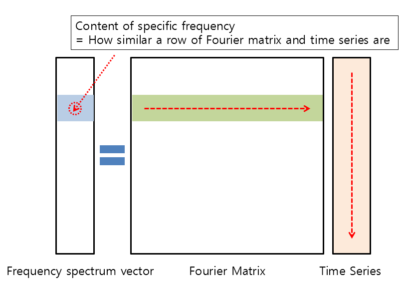
Figure 2. Frequency component vectors can be obtained by checking the similarity between the rows of the Fourier matrix and the time series vector.
So, what does each row of the Fourier matrix signify?
Meaning of the Fourier Matrix
In the article Geometric Interpretation of Euler’s Formula, the meaning of the following formula has been discussed:
\[e^{j\theta}=\cos(\theta) + j\sin(\theta)\]To understand the meaning of Equation (41), we can observe the value of the right-hand side, which represents the coordinates of a point on the complex plane that has rotated by $\theta$ radians from the origin along an arc.
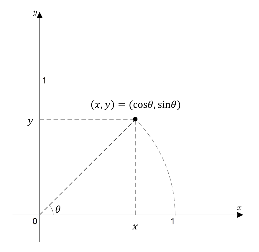
Figure 3. x+iy represented in the complex plane. In trigonometric form, it is cos(theta) + i sin(theta) with theta being the angle from the x-axis in radians.
In other words, $w$ in equation (40) is calculated as follows:
\[w = \exp\left(-j\frac{2\pi}{N}\right)\]This means that $w$ is the position of the first point obtained by dividing a circle into $N$ equal parts and rotating around the circle once in a clockwise direction.
Let’s consider the meaning of $w$ while examining the Fourier matrix for the case where $N=8$.
For $N=8$, the value of $w$ in the Fourier matrix is $w=\exp\left(-j\frac{2\pi}{8}\right)$. Representing this on the complex plane gives the following:
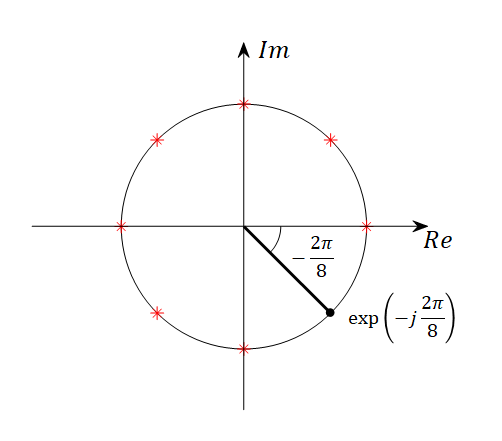
Figure 4. $\exp(-j 2\pi/8)$ represented on the complex plane. The red asterisks indicate the positions of $w$ to the power of 0, 2, 3, ..., and 7.
If we replace the complex numbers in the Fourier matrix with the phases indicated by the complex number $w$ on the unit circle, the resulting visualization would be as shown in Figure 5.
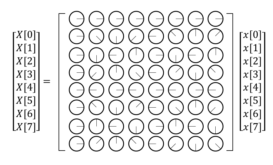
Figure 5. Visualization of the Fourier matrix for $N=8$. The visualization within the Fourier matrix represents the phase indicated by the complex number $w$.
Since both cosine and sine functions originate from the concept of rotation on a circle, we can think of the value of the phase obtained from the rotation as equivalent to the value of cosine or sine functions.
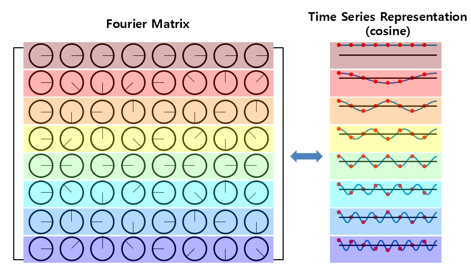
Figure 6. The phase of each complex element in the Fourier matrix, when replaced with sine functions
As seen in Figure 6, each row of the Fourier matrix represents a cosine function that starts from frequency 0 and goes up to multiples of the fundamental frequency.
Furthermore, if we consider the phase of the Fourier matrix with respect to sine functions,
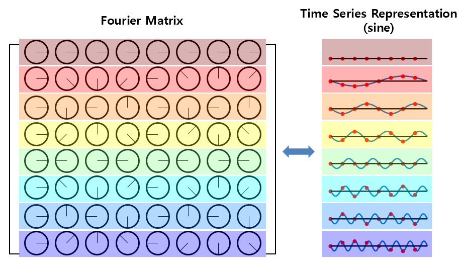
Figure 7. The phase of each complex element in the Fourier matrix, when replaced with sine functions
As seen in Figure 7, each row of the Fourier matrix also represents a sine function that starts from frequency 0 and goes up to multiples of the fundamental frequency.
In other words, the Fourier matrix used for calculating the Discrete Fourier Transform (DFT) consists of cosine and sine functions that are multiples of the fundamental frequency, and these functions form the real and imaginary parts, respectively, which are then multiplied with the original time-domain signal to obtain the result.
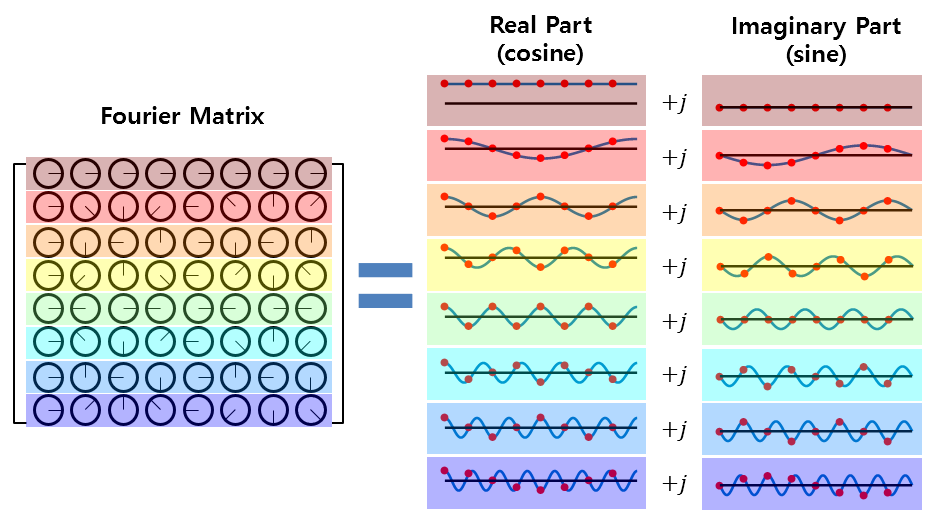
Figure 8. All values in the Fourier matrix are complex numbers, consisting of cosine and sine functions as their real and imaginary parts, respectively.
Characteristics of Fourier Matrix
Let’s now examine the characteristics of the Fourier matrix.
1. Columns of the Fourier matrix are orthogonal to each other
We can easily verify that the columns of the Fourier matrix are orthogonal to each other using a simple method.
The easiest way is to take the Hermitian operation1 on the Fourier matrix $F$ and then multiply it.
In other words, by taking the Hermitian operation of the Fourier matrix and multiplying it, we can confirm that the columns of the Fourier matrix are orthogonal to each other.
\[F^HF = \begin{bmatrix} 1 && 1 && 1 && \cdots && 1 \\ 1 && w^{*1} && w^{*2} && \cdots && w^{*(N-1)} \\ 1 && \vdots && \vdots && \ddots && \vdots \\ 1 && w^{*(N-1)} && w^{*(N-1)\cdot 2} && \cdots && w^{*(N-1)\cdot(N-1)}\end{bmatrix} \begin{bmatrix} 1 && 1 && 1 && \cdots && 1 \\ 1 && w^1 && w^2 && \cdots && w^{N-1} \\ 1 && \vdots && \vdots && \ddots && \vdots \\ 1 && w^{N-1} && w^{(N-1)\cdot 2} && \cdots && w^{(N-1)\cdot(N-1)}\end{bmatrix}\] \[=N\begin{bmatrix}1 && 0 && \cdots && 0 \\ 0 && 1 && \cdots && 0 \\ \vdots && \vdots && \ddots && \vdots \\ 0 && 0 && \cdots && 1\end{bmatrix} = N\cdot I\]Here, the superscript ‘*’ means complex conjugate.
As a result of equation (44), the columns of the Fourier matrix $F$ have the value of $N$ when taking the inner product with themselves, and have the value of 0 when taking the inner product with other columns, which confirms that each column is orthogonal to each other.
2. Inverse Fourier Matrix and Inverse Fourier Transform
Furthermore, through equations (43) and (44), we can determine that the inverse Fourier matrix is given by
\[F^{-1}=\frac{1}{N}F^H\]where $F^H$ represents the Hermitian transpose of the Fourier matrix.
In other words, the inverse Fourier matrix is obtained by taking the Hermitian transpose of the Fourier matrix and dividing it by $N$.
\[\begin{bmatrix}x[0]\\x[1]\\ \vdots \\ x[n-1]\end{bmatrix} = \frac{1}{N}\begin{bmatrix} 1 && 1 && 1 && \cdots && 1 \\ 1 && w^{*1} && w^{*2} && \cdots && w^{*(N-1)} \\ 1 && \vdots && \vdots && \ddots && \vdots \\ 1 && w^{*(N-1)} && w^{*(N-1)\cdot 2} && \cdots && w^{*(N-1)\cdot(N-1)}\end{bmatrix}\begin{bmatrix}X[0]\\X[1]\\ \vdots \\ X[N-1]\end{bmatrix}\]3. What Inverse Fourier Transform Tells Us
Let’s revisit the interpretation part based on column spaces in Another Perspective on Matrix Multiplication.
For example, for the following matrix:
\[\begin{bmatrix}1 & 2 \\ 3 & 4\end{bmatrix}\begin{bmatrix}x\\y\end{bmatrix}=\begin{bmatrix}3\\5\end{bmatrix}\]we can easily solve the system of linear equations as follows:
\[\begin{cases} x+2y = 3 \\ 3x+4y = 5 \end{cases}\] \[\Rightarrow x=-1, \text{ }y=2\]However, let’s think about this equation in the following way this time:
\[x\begin{bmatrix}1\\3\end{bmatrix}+y\begin{bmatrix}2\\4\end{bmatrix}=\begin{bmatrix}3\\5\end{bmatrix}\]As mentioned in the article Another Perspective on Matrix Multiplication, the interpretation of the above equation can also be done as follows:
Applying this idea to the Fourier matrix, the meaning of taking the inverse Fourier transform is as follows:
“Is there an N-dimensional time series vector within the vector space generated by the N columns of $F^{-1}$?”
“If so, how can we combine the column vectors of $F^{-1}$ to create the time series vector?”
In other words, what does this mean?
In other words, it reaffirms that all time series can be composed of a sum of sinusoidal waves, and the form of the time series depends on how the sinusoidal waves are combined.
-
Hermitian operator = Transpose + complex conjugate. ↩