Properties of the Determinant of a Matrix
To better understand Cramer’s Rule, it is helpful to have a good understanding of the following properties of the determinant of a matrix.
- The determinant of a matrix has the same meaning as the area of the parallelogram formed by the column vectors of the matrix.
For example, for any matrix
\[A=\begin{bmatrix}a & b \\ c & d\end{bmatrix}\]if we denote each column vector as $U$, $V$, respectively, then $\det(A)=ad-bc$ is equal to the area of the parallelogram formed by the column vectors as shown below:
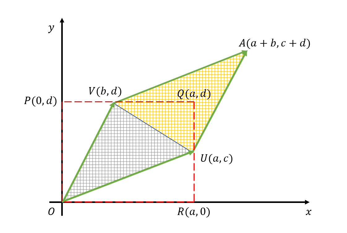
Figure 1. The value of the determinant is equal to the area of the parallelogram formed by the column vectors $U$ and $V$.
Therefore, if the vectors forming the parallelogram are parallel, then the area of the parallelogram is 0.
In other words, if the column vectors of matrix $A$ are linearly dependent, then the area of the parallelogram is 0, and $A$ does not have an inverse.
- If one column of the matrix $A$ is multiplied by a scalar $k$, then the value of the determinant is also multiplied by $k$.
In other words, the determinant satisfies the following property:
\[\det\left(\begin{bmatrix}a & k\cdot b \\c & k\cdot d\end{bmatrix}\right)=k\cdot\det\left(\begin{bmatrix}a & b \\ c & d\end{bmatrix}\right)\]This property is easy to understand by imagining one side of the parallelogram in Figure 1 being multiplied by $k$.
- Let $A_1, A_2, B_1, B_2, A_n$ be column vectors of a matrix and let $k_1, k_2$ be scalars. When representing the matrix using column vectors enclosed in $[]$, the determinant satisfies the following property:
Cramer’s Rule
Cramer’s rule is a formula that can be used to obtain solutions to equations like the one below:
Given an $n\times n$ matrix $A$ and an $n\times 1$ vector $b$, and letting $x=[x_1, x_2, \cdots, x_n]^T$,
\[Ax=b\]When this equation holds, each element $x_i$ of the solution $x$ is determined by the formula:
\[x_i = \frac{\text{det}(A^{rep}_{i})}{\text{det}(A)}\]where $A^{rep}_{i}$ is the matrix obtained by replacing the $i$th column of $A$ with the vector $b$.
In other words, for the equation $Ax=b$ as shown below,
\[Ax=b \iff \begin{bmatrix} a_{11} & \cdots & \color{red}{a_{1i}} & \cdots & a_{1n}\\ a_{21} & \cdots & \color{red}{a_{2i}} & \cdots & a_{2n}\\ \vdots & & \vdots & & \vdots \\ a_{n1} & \cdots & \color{red}{a_{ni}} & \cdots & a_nn \end{bmatrix} \begin{bmatrix}x_1 \\ x_2 \\ \vdots \\ x_n\end{bmatrix} = \begin{bmatrix}b_1 \\ b_2 \\ \vdots \\ b_n\end{bmatrix}\]The $i$-th element $x_i$ of vector $x$ is determined as follows.
\[x_i = \frac{\det(A_i^{rep})}{\det(A)}= \frac { \left|\begin{matrix} a_{11} & \cdots & \color{red}{b_{1}} & \cdots & a_{1n}\\ a_{21} & \cdots & \color{red}{b_{2}} & \cdots & a_{2n}\\ \vdots & & \vdots & & \vdots \\ a_{n1} & \cdots & \color{red}{b_{n}} & \cdots & a_nn \end{matrix}\right|} { \left|\begin{matrix} a_{11} & \cdots & a_{1i} & \cdots & a_{1n}\\ a_{21} & \cdots & a_{2i} & \cdots & a_{2n}\\ \vdots & & \vdots & & \vdots \\ a_{n1} & \cdots & a_{ni} & \cdots & a_nn \end{matrix}\right|}\]Proof of a Formula
Matrix $A$ can be seen as a stack of $n$ column vectors arranged side by side, as follows:
\[A=\begin{bmatrix} | & | & & | \\ A_1 & A_2 & \cdots & A_n \\ | & | & & | \end{bmatrix}\]Using the column notation of $A$, $Ax=b$ can also be written as:
By denoting each column of $A$ as
\[\begin{bmatrix} | \\ A_1\\ |\end{bmatrix}, \begin{bmatrix}| \\ A_2\\ |\end{bmatrix}, \cdots, \begin{bmatrix}| \\ A_n\\ |\end{bmatrix}\]and each element of $x$ as $x_1$, $x_2$, $\cdots$, $x_n$, we can write:
\[Ax=x_1\begin{bmatrix}| \\ A_1\\ |\end{bmatrix}+x_2\begin{bmatrix}| \\ A_2\\ |\end{bmatrix}+\cdots+x_n\begin{bmatrix}| \\ A_n\\ |\end{bmatrix} = b\]Let’s call the matrix obtained by replacing the $i$th column of $A$ with the vector $b$ as $A^{rep}_{i}$. In other words,
\[A^{rep}_{i} =\begin{bmatrix} | & | & & | & & | \\ A_1 & A_2 & \cdots & b & \cdots & A_n \\ | & | & & | & & | \end{bmatrix}\]where $b$ is inserted in the $i$th column.
For convenience, let’s use the following notation:
\[A^{rep}_{i} = [A_1, A_2, \cdots, b,\cdots,A_n]\]Note that this notation represents $A^{rep}_{i}$ with $b$ inserted in the $i$th column.
Now, let’s calculate the determinant of $A^{rep}_{i}$.
\[\text{det}(A^{rep}_{i}) = \text{det}\left([A_1, A_2, \cdots, b,\cdots,A_n]\right)\]Since $b$ can be expressed as $x_1A_1 + x_2A_2 + \cdots + x_nA_n$,
\[\Rightarrow \text{det}\left([A_1, A_2, \cdots, \color{red}{x_1A_1 + x_2A_2 + \cdots + x_nA_n},\cdots,A_n]\right)\]by the property of determinants,
\[\Rightarrow \color{red}{x_1} \text{det}\left([A_1, A_2, \cdots, \color{red}{A_1},\cdots,A_n]\right) \\ \quad + \color{red}{x_2} \text{det}\left([A_1, A_2, \cdots, \color{red}{A_2},\cdots,A_n]\right) \\ \vdots \\ \quad + \color{red}{x_n} \text{det}\left([A_1, A_2, \cdots, \color{red}{A_n},\cdots,A_n]\right)\] \[=\sum_{j=1}^{n}\color{red}{x_j} \text{det}\left([A_1, A_2, \cdots, \color{red}{A_j},\cdots,A_n]\right)\]If there exists a column vector in a matrix that is not linearly independent, then the value of the determinant of the matrix is 0.
Therefore, the above equation is only non-zero when $j=i$, and in all other cases it becomes 0.
Therefore,
\[\Rightarrow x_i \text{det}\left([A_1, A_2, \cdots, A_i, \cdots, A_n]\right)\]However, the matrix $[A_1, A_2, \cdots, A_i, \cdots, A_n]$ is the same as the original $A$ matrix, so the above equation is
\[\Rightarrow x_i \text{det}(A)\]Therefore, comparing with the original equation,
\[\text{det}(A^{rep}_{i})=x_i\text{det}(A)\]thus,
\[x_i = \frac{\text{det}(A^{rep}_{i})}{\text{det}(A)}\]can be inferred.
Geometric Interpretation
Prerequisites
To understand the geometric interpretation of Cramer’s rule, it is recommended to have knowledge of the following:
- Another perspective on matrix multiplication
- Geometric interpretation of determinants
- Area of a parallelogram = base x height
Geometric Interpretation
The geometric interpretation of Cramer’s rule can be interpreted with only two facts: that the determinant of a matrix is equal to the area of the parallelogram formed by two vectors and that the area of the parallelogram can be calculated as the product of the base and height.
Consider the simple matrix-vector multiplication below:
\[Ax=b\] \[\Rightarrow \begin{bmatrix}a & b \\ c & d\end{bmatrix}\begin{bmatrix}x_1 \\ x_2\end{bmatrix}=\begin{bmatrix}b_1 \\ b_2\end{bmatrix}\]As shown in the Another perspective on matrix multiplication article, we can also express the product of the above matrix and vector as follows:
\[x_1\begin{bmatrix}a\\c \end{bmatrix}+x_2\begin{bmatrix}b\\d \end{bmatrix}=\begin{bmatrix}b_1 \\ b_2 \end{bmatrix}\]This can be represented graphically as follows:
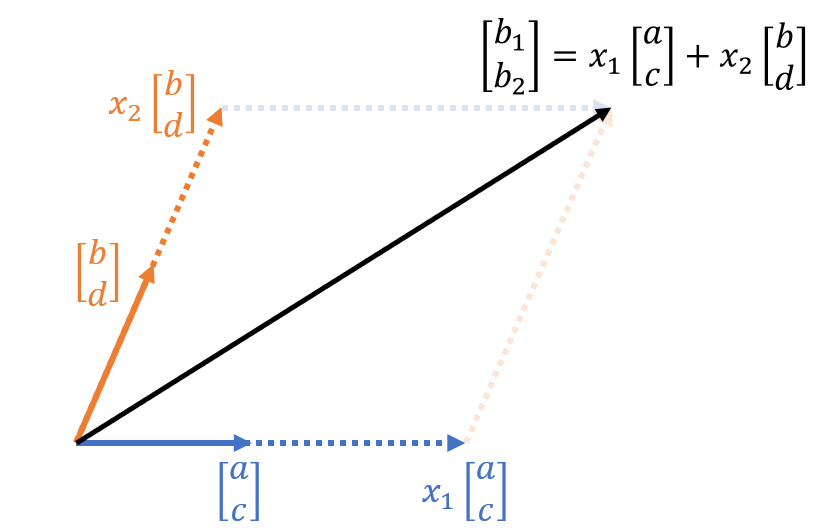
Figure 1. Graphical representation of the product of the matrix and vector in equation (18)
At this point, let’s observe three parallelograms.
The first is a parallelogram formed by the column vectors of matrix $A$ in equation (16).
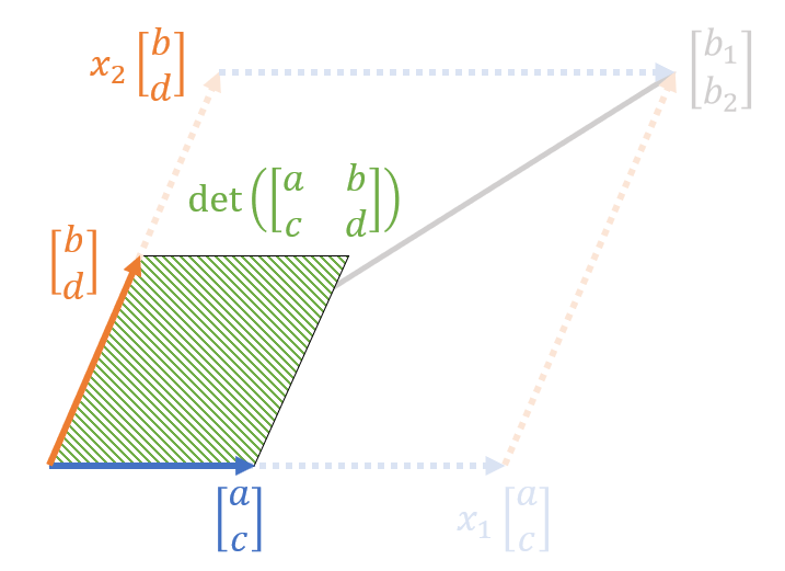
Figure 2. Parallelogram composed of the column vectors of matrix $A$ in equation (16)
The area of the parallelogram can be expressed as the value of the determinant, as we saw in the geometric interpretation of the determinant.
The second parallelogram can be defined as a parallelogram consisting of a vector obtained by multiplying $[b, d]^T$ by $x_2$ and the two column vectors of $[a, c]^T$.
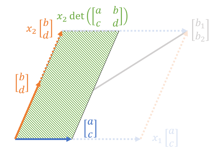
Figure 3. Parallelogram composed of a vector obtained by multiplying $[b, d]^T$ by $x_2$ and the two column vectors of $[a, c]^T$
The area of this parallelogram can be easily calculated as follows:
\[det\left(\begin{bmatrix}a & x_2 b \\ c & x_2 d\end{bmatrix}\right)\]We can see that the parallelogram observed in Figure 3 is x_2 times larger than the parallelogram seen in Figure 2.
Alternatively, by the property of determinants, we can write:
\[\Rightarrow x_2 \ det\left(\begin{bmatrix}a & b \\ c & d\end{bmatrix}\right)\]On the other hand, the third parallelogram we will observe is shown in Figure 4 below.
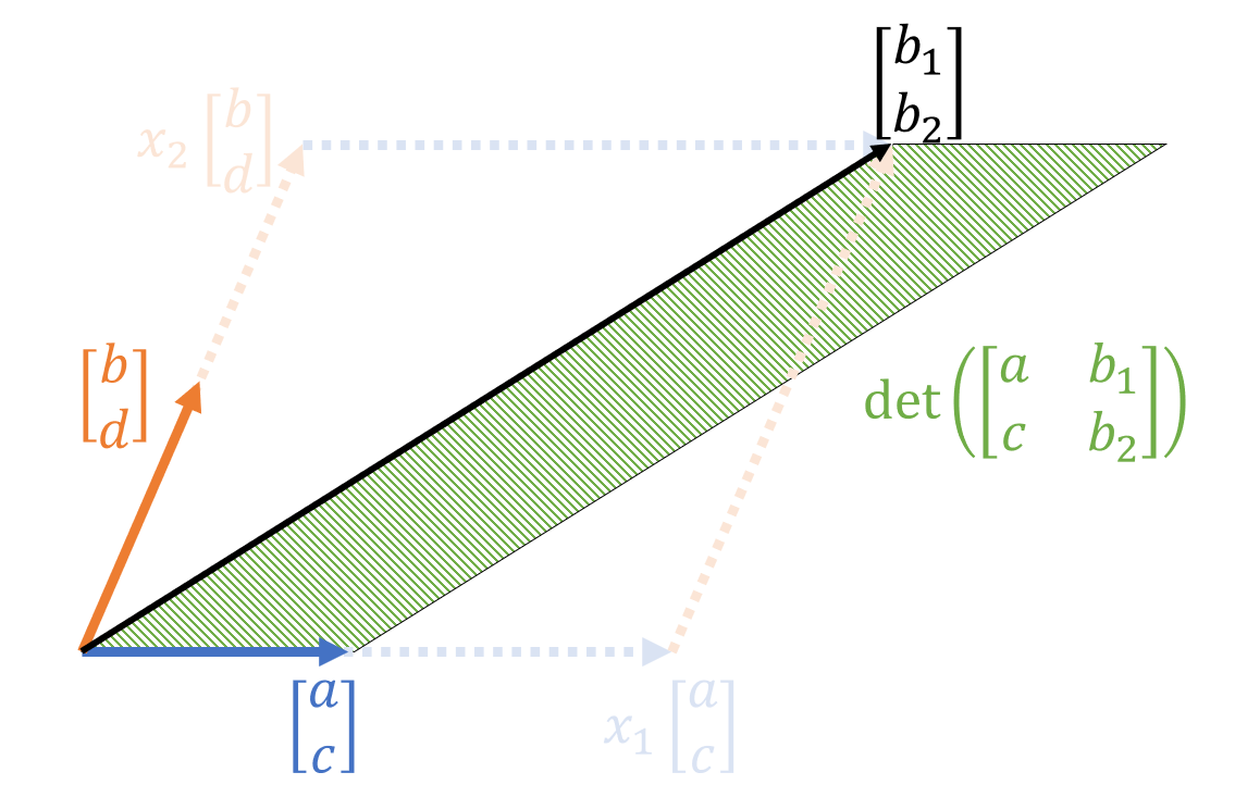
Figure 4. Parallelogram composed of the vectors $[a,c]^T$ and $[b_1, b_2]^T$
The area of the parallelogram in Figure 4 can be expressed using the determinant as follows:
\[det\left(\begin{bmatrix}a & b_1\\ c & b_2\end{bmatrix}\right)\]Interestingly, the areas of the parallelograms in Figure 3 and Figure 4 are the same. This is because the length of the base does not change and the heights of the two parallelograms are the same.
Therefore,
\[x_2 \ det\left(\begin{bmatrix}a & b \\ c & d\end{bmatrix}\right)=det\left(\begin{bmatrix}a & b_1\\ c & b_2\end{bmatrix}\right)\]which means that
\[x_2 = \frac{det\left(\begin{bmatrix}a & b_1\\ c & b_2\end{bmatrix}\right)}{det\left(\begin{bmatrix}a & b \\ c & d\end{bmatrix}\right)}\]We can confirm this in the same way for $x_1$.
Last but not least, this result corresponds to Cramer’s rule