Linear Regression with Gradient Descent
What Linear Regression is about: How can we draw a trend line that best explains a large number of points?

Regression Analysis from the Perspective of Linear Algebra

※ If you’re curious about optimization-related content, you can skip the section on Regression Analysis from the Perspective of Linear Algebra.

Prerequisites

To understand this content, it’s recommended that you know about the following:

• Basic operations of vectors (scalar multiplication, addition)
• Meaning of row vectors and inner product of vectors
• Relationship between the four major subspace

Finding solutions using linear systems of equations

You may have learned about systems of linear equations in middle school.

A system of linear equations refers to a set of equations that include two or more unknowns, and in most cases in middle and high school courses, we solved two-variable linear equations.

The general form of a system of equations can be written as follows.

\[\begin{cases} ax + by = p \\ cx + dy = q \end{cases}\]

In this post, we will consider linear regression by finding an appropriate solution for cases where we have more data than unknowns.

For example, suppose we have the following three data points.

\[(-1, 0),\text{ }(0, 1),\text{ }(0, 3)\]

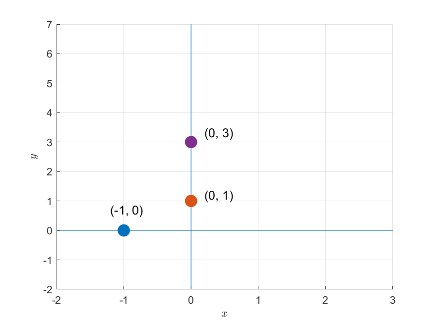
Figure 1. Three given data points

Suppose we obtained these three data points through a model like $f(x) = mx+b$. Then, we can formulate a system of equations consisting of three equations as follows:

\[f(-1) = -m + b = 0\] \[f(0) = 0 + b = 1\] \[f(0) = 0 + b = 3\]

Representing this using matrices and vectors, we get:

\[(Ax = b) \Rightarrow\begin{bmatrix}-1 && 1 \\ 0 && 1 \\ 0 && 1\end{bmatrix}\begin{bmatrix}m \\ b\end{bmatrix} = \begin{bmatrix}0\\1 \\ 3 \end{bmatrix}\]

From a geometric perspective, solving this matrix is equivalent to finding a line that passes through all three data points, as shown in Figure 1.

No matter how we position the line on the 2D plane, we cannot find a line that passes through all three points simultaneously.

In other words, this problem is unsolvable because there is no solution.

Linear Algebraic Perspective

From a linear algebraic perspective, solving a system of equations is equivalent to solving a matrix equation like:

\[A\vec{x} = \vec{b}\]

Expressing both the vector and matrix as column vectors, and splitting the two elements of $\vec{x}$, we get:

\[\Rightarrow \begin{bmatrix} | & | \\ \vec{a}_1 & \vec{a}_2 \\ | & | \end{bmatrix}\begin{bmatrix}x_1 \\ x_2\end{bmatrix} = \begin{bmatrix}\text{ } | \text{ } \\ \text{ } \vec{b} \text{ }\\\text{ } | \text{ }\end{bmatrix}\]

Then, the equation can be thought of as follows:

\[\Rightarrow x_1\begin{bmatrix} | \\ \vec{a}_1 \\ | \end{bmatrix} + x_2\begin{bmatrix} | \\ \vec{a}_2 \\ | \end{bmatrix} = \begin{bmatrix}\text{ } | \text{ } \\ \text{ } \vec{b} \text{ }\\\text{ } | \text{ }\end{bmatrix}\]

In other words, it is like answering the question of what the appropriate combination ratios $x_1$ and $x_2$ are to obtain $\vec{b}$ by combining the column vectors $\vec{a}_1$ and $\vec{a}_2$.

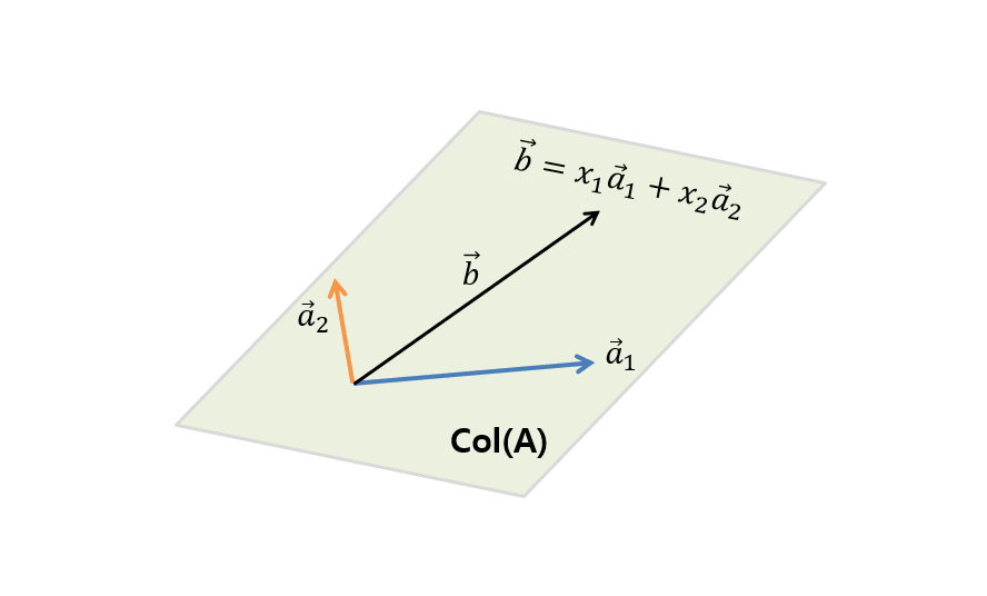
Figure 2. To find the vector $\vec{b}$ contained in the column space $col(A)$ of A, which is the span of the column vectors ($\vec{a}_1$, $\vec{a}_2$) forming the columns of A, how much should $\vec{a}_1$ and $\vec{a}_2$ be combined?

However, in order to obtain $\vec{b}$ by combining $\vec{a}_1$ and $\vec{a}_2$, $\vec{b}$ must be one of all possible combinations that can be obtained by combining $\vec{a}_1$ and $\vec{a}_2.

In other words, $\vec{b}$ must be contained in the span of $\vec{a}_1$ and $\vec{a}_2$. This is the condition for finding a solution.

Finding the optimal solution

As they say, something is better than nothing. If you cannot find the exact answer as in the problem like in Figure 1, you should at least find something that is as close to the answer as possible.

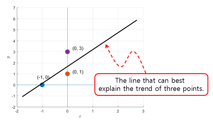
Figure 3. Let's draw a line that can best describe the trends of the three points.

Here, the process of finding a line that can well represent the trend of three points can be thought of as the process of finding the solution ($\vec{b}$) that is closest to the answer within the column space of the matrix A when the solution does not exist in the column space.

In fact, if you draw $\vec{a}_1$, $\vec{a}_2$, the column space generated by these two vectors, and $\vec{b}$ directly in Figure 1 or Figure 3 problems, it would look like the following:

Figure 4. Column space represented by the span of two vectors, $[-1, 0, 0]^T$ (blue) and $[1, 1, 1]^T$ (orange), and a vector $[0, 1, 3]^T$ (purple) that is not included in this space.

If we abstract the content of Figure 4 a bit more, we get Figure 5 below.

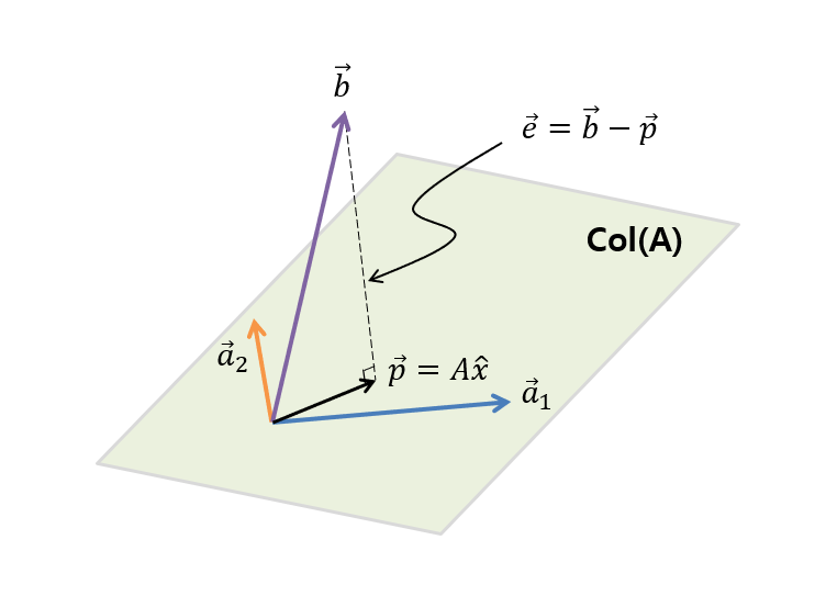
Figure 5. Column space $col(A)$ of matrix A, which is the span of the column vectors ($\vec{a}_1$, $\vec{a}_2$) that make up the columns of A, and a vector $\vec{b}$ that is not in the column space.

As you can see in Figure 5, $\vec{b}$ is not included in the column space of $\vec{a}_1$ and $\vec{a}_2$. And as shown in Figure 5, the closest vector to $\vec{b}$ that can be obtained through a linear combination of $\vec{a}_1$ and $\vec{a}_2$ is the projection $\vec{p}$ of $\vec{b}$ onto the column space (col(A)), and by calculating this $\vec{p}$, we can find out how much we should linearly combine $\vec{a}_1$ and $\vec{a}_2$ ($\hat{x}$) to get as close as possible to $\vec{b}$.

Then, if we define the difference vector between the original solution $\vec{b}$ and the projection vector $\vec{p}$ as $\vec{e}$, it will be orthogonal to any vector in the matrix $A$, so the following equation holds:

\[A\cdot\vec{e} = \begin{bmatrix} | & | \\ \vec{a}_1 & \vec{a}_2 \\ | & | \end{bmatrix}\cdot\vec{e} = 0\]

Here, ‘$\cdot$’ denotes inner product.

In other words, if we calculate the inner product, we get:

\[A^Te = A^T(\vec{b}-A\hat{x}) = 0\] \[\Rightarrow A^T\vec{b}-A^TA\hat{x} = 0\] \[\Rightarrow A^TA\hat{x} = A^T\vec{b}\] \[\therefore \hat{x}=(A^TA)^{-1}A^T\vec{b}\]

Explanation Using Basic Subspaces

In Figure 5, the vector $\vec{e}$ is orthogonal to all vectors in the column space. Based on what we saw in the Four Fundamental Subspaces, we can conclude that $\vec{e}$ is a vector in the left nullspace.

In other words, the vector $\vec{b}$ is located in a space that can only be composed of basis vectors that can be created from the column space and left nullspace, and $\vec{p}$ represents the vector that is closest to the column space, while $\vec{e}$ represents the vector in the left nullspace.

The relationship between the fundamental subspaces of linear regression, viewed from a linear algebra perspective, is shown in Figure 6 below.

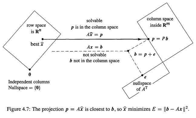
Figure 6. Relationships between basic subspaces in linear regression viewed from a linear algebra perspective.
Image source: Introduction to Linear Algebra, Gilbert Strang

A nullspace of ${0}$ means that if the nullspace is not the zero vector space, the function would have an infinitely large slope, making it impossible to define the function. Therefore, when using a linear regression model to obtain a function, we exclude cases where the nullspace is not the zero vector space.

Actual Calculation

We can set $A$ and $b$ as shown below in MATLAB and calculate $\hat{x}$.

A = [-1, 1; 0, 1; 0, 1];
b = [0; 1; 3];

x_hat = inv(A'*A)*A'*b;

The result is as follows.

x_hat =

     2
     2

In other words, it means that the line with a slope of 2 and an intercept of 2, as shown in Figure 7 below, is the point that can best explain the trend of the three points seen in Figures 1 and 3.

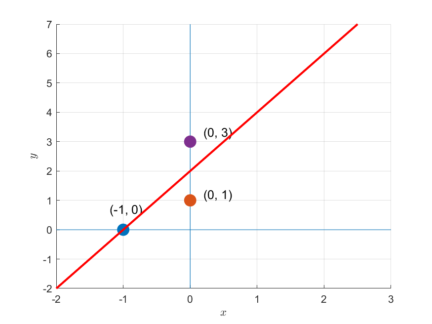
Figure 7. The optimal regression equation for the data seen in Figures 1 and 3.

Linear regression from the perspective of optimization problems

※ If you are curious about linear algebra-related topics, you can skip the part $\lt$Linear regression from the perspective of optimization problems$\gt$.

Prerequisites

To understand linear regression from the perspective of optimization problems, it is recommended that you have knowledge of the following:

• The meaning of gradient
• Gradient descent

Introduction to linear regression from the perspective of optimization problems

Linear regression from the perspective of optimization problems can start with setting a model for the data.

For example, let’s say we have data with two features as shown in the figure below.

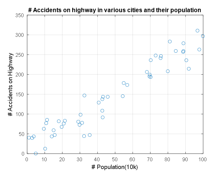
Figure 8. A pair of features that are correlated with each other

This data represents the population and number of traffic accidents in each state, represented on the x and y axes respectively.

We want to assume a model for this data.

Looking at the shape of the data, it seems that there is no problem modeling this data with a linear model.

That is, we can say that our model is a first-degree function with two parameters, as follows:

\[y = f(x) = ax+b\]

However, how should we determine the parameters $a$ and $b$ of this model? In other words, what line explains our data best?

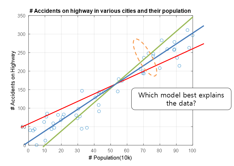
Figure 9. Which model explains the relationship between the features of this data the best?

Defining the Cost Function

Here, we should be able to determine which line best explains our data.

When we say “best explains,” we could define it as having the least difference or gap between the model and the data.

In other words, we could say that the model with the smallest average error for the entire data set is a better model. We can define the error ($e$) for a particular $i$-th data point as follows:

If we define the $y$-axis feature value from our linear model as $\hat{y}_i$ and the given $y$-axis feature value from the data as $y_i$, we can think of it as:

\[e_i = \hat{y_i} - y_i\]

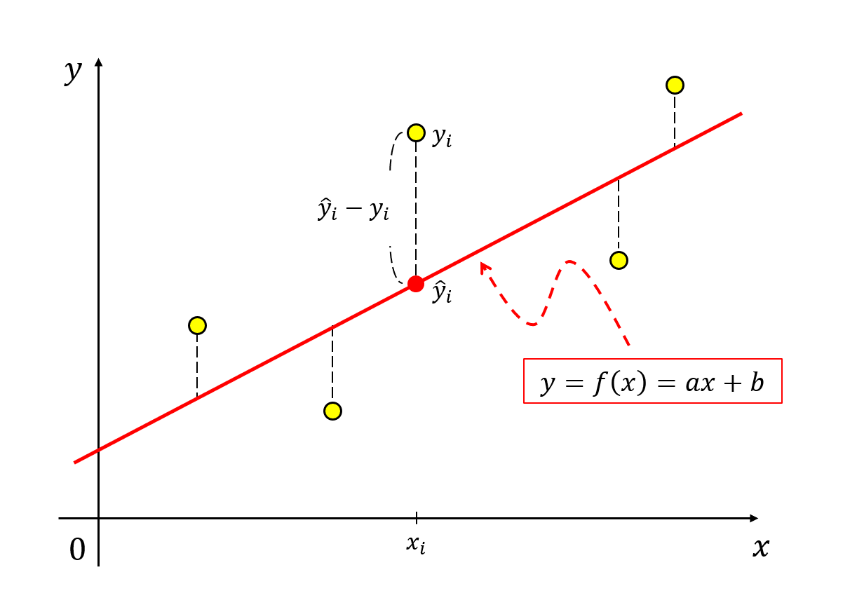
Figure 10. Difference between the predicted value of the linear model and the actual data.

If we want to avoid worrying about the sign of the error, we can define it as follows:

\[e_i = (\hat{y_i} - y_i)^2\]

Later on, we will differentiate the error function, so it would be a good idea to define it as follows in order to simplify the differentiation process:

\[e_i = \frac{1}{2}(\hat{y_i} - y_i)^2\]

Now, if we assume that there are a total of $N$ data points, we can calculate the average error for all data points as follows:

\[E = \frac{1}{N}\sum_{i=1}^Ne_i = \frac{1}{N}\sum_{i=1}^N\frac{1}{2}(\hat{y_i} - y_i)^2 = \frac{1}{2N}\sum_{i=1}^{N}(\hat{y_i} - y_i)^2\] \[=\frac{1}{2N}\sum_{i=1}^{N}\left(ax_i+b-y_i\right)^2\]

Here, our model is $f(x) = ax+b$, so we calculated $\hat{y}_i$ as $ax_i + b$.

Visualization of the Cost Function

The $E$ previously calculated is what is called the ‘cost function’, which can be seen as having good explanatory power for the data as the cost function value becomes smaller.

Since our data $x_i$ and $y_i$ are given, it is also possible to view the cost function $E$ as a function of $a$ and $b$.

That is,

\[E=f(a, b) = \frac{1}{2N}\sum_{i=1}^{N}\left(ax_i+b-y_i\right)^2\]

can be written.

Then, finding a regression model that explains the data well can be thought of as finding $a$ and $b$ that minimize $E$, that is, reducing the problem to finding the minimum value of $E$.

If we visualize this, we can say that in the space where slope (i.e., $a$ above) and intercept (i.e., $b$ above) are the domain, the cost function $E$ exists as a scalar function, as shown in Figure 11 below.

Figure 11. Cost function and its minimum value (star) in the space where slope and intercept are the domain
※ The parameters of the cost function are all normalized for visualization.

That is, how can we find the minimum value shown in Figure 11?

Calculation of Minimum Cost Function Using Gradient Descent

There are many ways to find the minimum value of a function, but generally, gradient descent is most commonly used to solve the problem of finding the minimum value of the cost function for regression models.

To briefly review gradient descent, it can be said to be a mathematical algorithm that takes one step at a time in the steepest direction when going downhill from a high place to a low place on a steep path.

Considering the meaning of gradient, it should be noted that the gradient is defined as the direction in which the slope is ‘increasing.’

If we look at the following figure and start the gradient descent algorithm at the point represented by the black dot, we can think of the direction of the gradient as the red arrow.

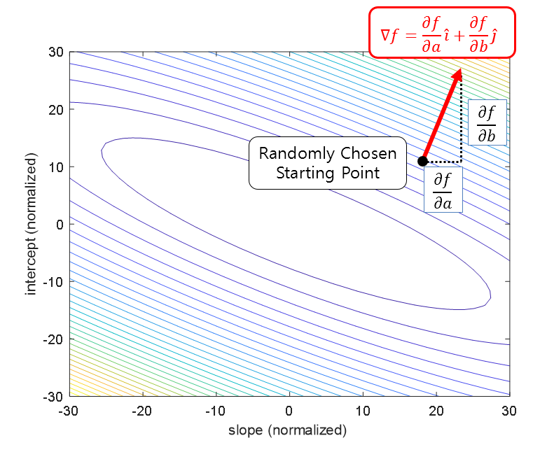
Figure 12. In the function space where the domain is $a$ and $b$ (slope and intercept in this case) and the height is the value of the cost function, the direction of the gradient at an arbitrary point is the direction in which the function value increases.

Therefore, since the direction of the gradient is the direction in which the function ‘increases’, we can update the positions of $a$ and $b$ step by step in the opposite direction. Eventually, we can move $a$ and $b$ to the location of the minimum value (denoted by a star) of the cost function $E=f(a,b)$.

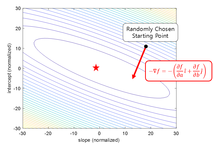
Figure 13. In the function space where the domain is $a$ and $b$ (slope and intercept in this case) and the height is the value of the cost function, if we update the positions of $a$ and $b$ in the opposite direction of the gradient at an arbitrary point, we can eventually find the $a$ and $b$ that minimize the cost function.

That is, we can set the parameters $a$ and $b$ to arbitrary values and update them in the function $f(a,b)$ that we want to find.

We can update the vector $[a, b]^T$ as follows:

\[\begin{bmatrix}a\\b\end{bmatrix}:=\begin{bmatrix}a\\b\end{bmatrix}-\alpha\nabla f(a, b)\]

Here, $\alpha$ is called the learning rate or step size, and it is a small number such as $0.1$ or $0.001$.

Expanding this, we have:

\[a := a - \alpha \frac{\partial f}{\partial a}\] \[b := b - \alpha \frac{\partial f}{\partial b} % Equation 24\]

Figure 14. The process of finding the minimum value of the cost function using gradient descent.
※ All parameters of the cost function have been normalized for visualization purposes.