Heat Equation

According to Wikipedia, the heat equation is a second-order partial differential equation that describes the process of conduction of properties such as heat over time.

Let’s exclude the complex term ‘second-order partial differential equation’ for now (it simply means that we took derivatives twice). The important keywords here are ‘time’ and ‘conduction’ with respect to time. Time is literally time, and ‘conduction’ refers to the spreading in space.

From this, we can infer that the heat equation involves one or more variables. The heat equation can be understood as a function that takes time and space as input and outputs heat.

When we talk about ‘space’, we usually think of three-dimensional space, but let’s consider a function that includes time in one-dimensional space for our understanding of the heat equation.

Intuition of the Heat Equation

To understand the heat equation, let’s consider a steel rod that has been heated to some extent, as shown in Figure 1.

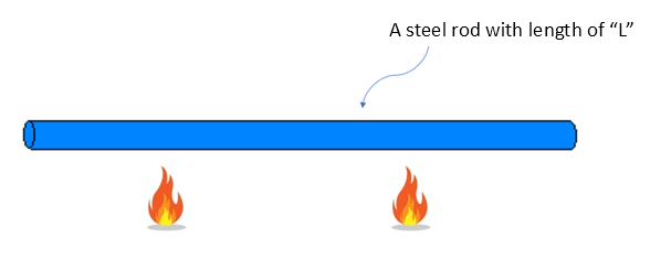
Figure 1. Let's imagine that the middle part of the steel rod has been heated for some time.

Then, if we denote the temperature¹ with respect to the length of the rod as $u(x)$, the distribution of $u(x)$ would roughly look like the following:

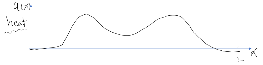
Figure 2. Distribution of temperature with respect to the length of the steel rod.

In other words, the heated areas would have increased in temperature, while the unheated areas would not have experienced such a significant temperature rise.

If we leave the situation in Figure 2 without further changes in external temperature, how would the situation progress?

In general, we can think that areas with higher temperature would decrease in temperature, while areas with lower temperature would increase in temperature.

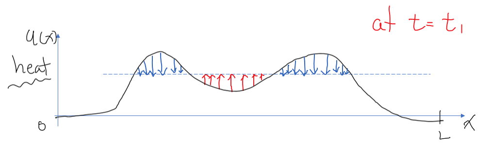
Figure 3. Changes over time. The red arrows represent temperature increase, while the blue arrows represent temperature decrease.

However, looking at Figure 3, we can see that it may not always be the case. The areas marked by red arrows may have higher temperature compared to the end point (x=0 or x=L) of the iron rod, but due to relatively higher temperature in the surrounding areas (indicated by blue arrows), the temperature actually increases.

In other words, the most important point to note is as follows:

Temperature changes due to relative temperature difference with the surrounding space.

In other words, if the surrounding temperature is high, the temperature increases, and if the surrounding temperature is low, the temperature decreases.

Furthermore, the faster the surrounding temperature is, the faster the temperature will increase, and the lower the surrounding temperature, the faster the temperature will decrease.

How can we mathematically express this?

The term ‘faster’ is related to speed, and the relationship with the ‘surrounding values’ can be thought of in terms of convexity and concavity. Here, ‘convex’ and ‘concave’ can be expressed in terms of second derivative coefficients.

Second Derivative Coefficients and Convexity, Concavity

You may have heard of the term ‘point of inflection’ during your high school days. The point of inflection refers to the point where the second derivative becomes 0, and the state changes from being convex upwards to concave downwards, or vice versa.

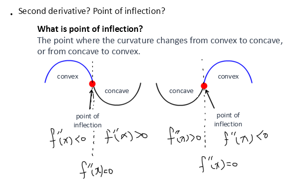
Figure 4. The point of inflection represents the moment when the state changes from convex to concave or vice versa.

In other words, mathematically, “concave up” can be written as

\[f''(x) < 0\]

and “concave down” can be written as

\[f''(x) > 0\]

Let’s remember this fact.

Meaning of Heat Equation

If we think about the meaning of the heat equation, we said that when the surrounding temperature is high, the temperature will rise quickly, and when the surrounding temperature is low, the temperature will drop quickly.

Our temperature distribution $u$ is a function of time and space, so we can write it as

\[u = f(x,t)\]

The change (velocity) of the temperature distribution with respect to time is denoted as

\[\frac{\partial u}{\partial t}\text{ or } u_t\]

Also, the degree to which the surrounding temperature is high or low can be expressed using second-order derivatives as

\[\frac{\partial^2u}{\partial x^2}\text{ or }u_{xx}\]

The rate of change of temperature is proportional to the degree of high or low surrounding temperature, so we can say

\[u_t \propto u_{xx}\]

Using the proportionality constant $k$, we can express it as

\[u_t = k u_{xx}\]

And this is the one-dimensional heat equation.

MATLAB demo 1: Example of a Metal Rod

Figure 5 shows a simulation of the temperature change in a metal rod discussed so far.

It can be observed that the temperature changes more rapidly in regions where the rod is more convex or concave.

Figure 5. Simulation of the temperature change in a metal rod

The 3D plot below displays the temperature change $u(x, t)$ of the metal rod in a three-dimensional space.

MATLAB demo 2: Example of a Steel Plate

So far, we have discussed examples of heat wave equations in one-dimensional space. In this example, we simulated a heat wave equation in two-dimensional space.

The scenario assumed is the simulation of how heat spreads in a steel plate after being heated with a lighter for one second and then no longer receiving any additional heat.

Figure 6. Simulation of the temperature change in a steel plate

It can be observed that, as before, regions with higher temperatures compared to their surroundings experience a more rapid decrease in temperature.

Wave Equation

The wave equation is a second-order partial differential equation used to describe phenomena such as sound waves, electromagnetic waves, and water waves. However, the wave equation referred to here is different from Schrödinger’s wave equation.

Understanding the meaning of the heat equation makes it much easier to understand the meaning of the wave equation.

Intuition of the Wave Equation

While the heat equation relates convexity and speed, the wave equation relates convexity and “force”. In other words, the more convex it is, the more force it experiences.

Mathematically, it can be expressed as follows:

\[\frac{\partial^2 u}{\partial t^2} = c^2 \frac{\partial^2 u}{\partial x^2}\]

or

\[u_{tt} = c^2 u_{xx}\]

Here, $c^2$ is a positive constant.

In other words, the left-hand side represents the term related to “acceleration” and the right-hand side represents the term related to “convexity”.

For example, when representing the form of waves and the forces acting on a rope placed in one-dimensional space, it can be shown as follows:

Figure 7. The 'force' experienced varies constantly with the convexity of the wave.
Source: Meaning of Vector Wave Equation, StackExchange

Simulation: Waves in 1D Space

The function of the wave equation can also be thought of as a function with 2-dimensional inputs, just like the function of the heat equation.

In other words, it can be expressed as a function of time and space (in this case, along the x-axis of the rope).

The movement of waves, as shown in Figure 7, can be represented in 3-dimensional space as follows:

Simulation: Water Waves in 2D Space

The MATLAB simulation below demonstrates water waves in 2-dimensional space. ¹

The assumed scenario is that a wave source periodically emits waves from the central point, and we observe how the waves propagate in the surrounding area.

Also, the space is bounded by walls, so we set the boundary condition such that the waves are reflected back.

Figure 8. Simulation of waves in 2D space