What probability density function with what mean value could these samples have been drawn from?
adapted from the Seeing Theory's amazing visualization of MLE
Definition of Maximum Likelihood Estimation
Maximum Likelihood Estimation (MLE) is a parametric data density estimation method that estimates parameters $\theta = (\theta_1, \cdots, \theta_m)$ from a probability density function $P(x|\theta)$ with observed sample data set $x = (x_1, x_2, \cdots, x_n)$.
Of course, just by reading this definition, it is impossible to understand what MLE is, so let’s look at an example to learn more about MLE.
Toy example of MLE
To understand the key idea of MLE, let’s consider a very simple toy example.
Let’s assume we have obtained the following 5 data points:
\[x = \lbrace1,4,5,6,9\rbrace\]At this point, looking at the following graph, which curve is more likely to have generated the data $x$, the orange curve or the blue curve?
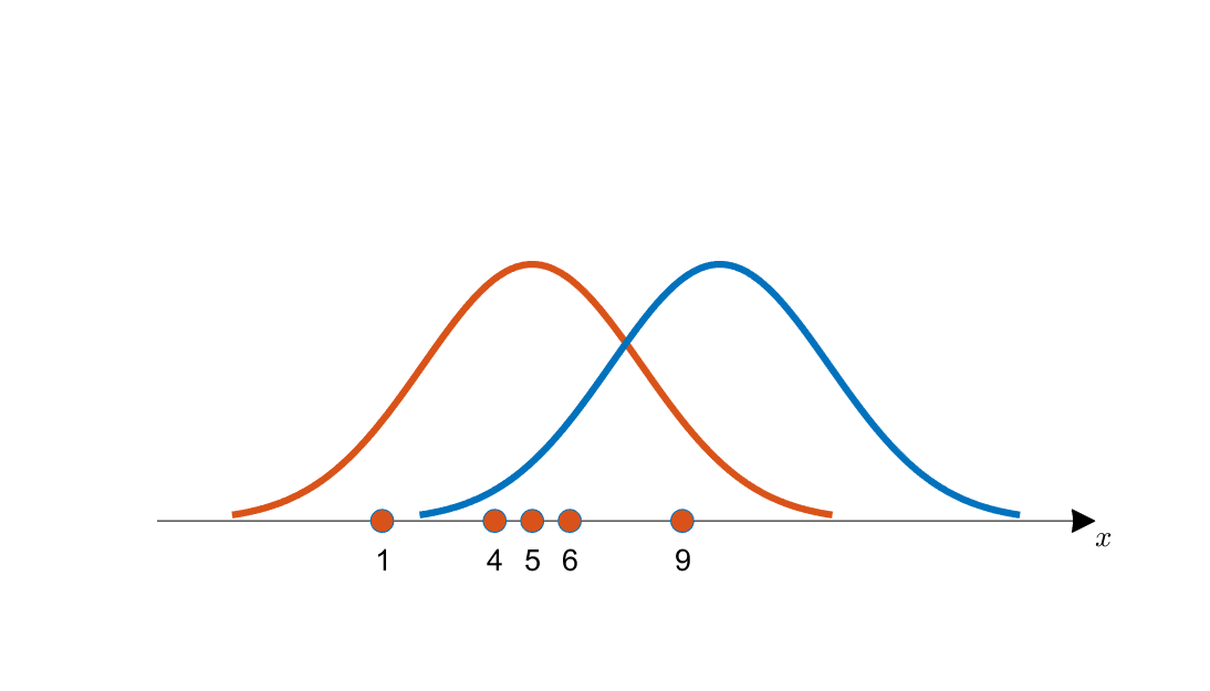
Figure 1. Observed data and two candidate distributions for estimation (indicated by orange and blue curves respectively)
Even by visually inspecting, it seems more likely that the data points were generated from the orange curve rather than the blue curve.
This is because the distribution of the acquired data points appears to align more with the center of the orange curve.
From this example, we can see that by observing the data, we can estimate the characteristics of the distribution from which the data was generated. In this case, we assumed that the distribution is a normal distribution, and we wanted to estimate the mean of the distribution.
Now let’s understand more specifically how to estimate the characteristics of this distribution precisely using mathematical methods.
Likelihood function
To discuss the mathematical estimation methods mentioned earlier, let’s talk about the contribution of likelihood from the data.
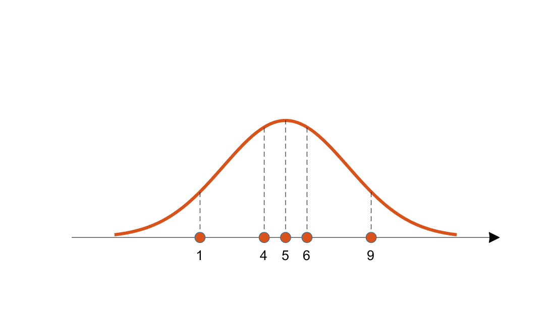
Figure 2. The height of the dotted lines represents the likelihood contribution of each data point for the orange candidate distribution.
Likelihood is simply the probability that the data we obtained came from this distribution.
To numerically calculate this likelihood, we can multiply the heights (i.e., likelihood contributions) of the data points for the candidate distribution, obtained from each data sample.
Multiplying instead of adding the calculated heights is due to the assumption that all data samples are independent events that occur sequentially.
By calculating this likelihood for all possible candidates and comparing them, we can obtain the probability distribution that best explains the data we obtained.
Mathematically, the likelihood discussed so far can be expressed more formally as follows:
The joint probability density function of the entire sample set as shown below is called the likelihood function.
\[P(x|\theta) = \prod_{k=1}^{n}P(x_k|\theta)\]It is most reasonable to consider the value of $\theta$ that maximizes the result of the above equation as the estimated value $\hat{\theta}$.
The likelihood function is often used in the form of the log-likelihood function $L(\theta | x)$ as shown below, using the natural logarithm for convenience in calculations.
\[L(\theta| x) = \log P(x|\theta) = \sum_{i=1}^{n}\log P(x_i | \theta)\]Method to find the maximum value of the likelihood function
In the end, Maximum Likelihood Estimation can be considered as a method to find the maximum value of the likelihood function.
Since the logarithm function is a monotonically increasing function, finding the maximum value of the likelihood function is equivalent to finding the maximum value of the log-likelihood function, and both cases have the same input values for the function’s domain.
Therefore, it is common to find the maximum value of the log-likelihood for convenience in calculations.
The most common method to find the maximum value of a function is to use derivative coefficients.
In other words, by partial differentiating with respect to the parameter $\theta$ we want to find, and finding the value of $\theta$ that makes the derivative equal to 0, we can find the $\theta$ that maximizes the likelihood function.
\[\frac{\partial}{\partial \theta}L(\theta|x) = \frac{\partial}{\partial \theta}\log P(x|\theta) = \sum_{i=1}^{n}\frac{\partial}{\partial\theta}\log P(x_i|\theta) = 0\]A more complex example of Maximum Likelihood Estimation (Estimation of population mean and population variance)
Let’s consider estimating the population mean $\mu$ and population variance $\sigma^2$ of a normal distribution when we have a sample $x_1, x_2, \cdots, x_n$ extracted from it. As you may already know, the estimated value of the population mean using the sample is given by:
\[\hat{\mu} = \frac{1}{n}\sum_{i=1}^{n}x_i\]and the estimated value of the population variance is given by:
\[\hat{\sigma}^2 = \frac{1}{n}\sum_{i=1}^{n}\left(x_i-\mu\right)^2\]Let’s confirm these estimators using the Maximum Likelihood Estimation (MLE) method.
Assuming that each sample is extracted from a normal distribution, the probability density function (pdf) of each sample is given by:
\[f_{\mu, \sigma^2}(x_i) = \frac{1}{\sigma\sqrt{2\pi}} \exp\left(-\frac{(x_i-\mu)^2}{2\sigma^2}\right)\]where $x_1, x_2, \cdots, x_n$ are assumed to be independently sampled. Then, the likelihood is given by:
\[P(x|\theta) = \prod_{i=1}^{n}f_{\mu, \sigma^2}(x_i) = \prod_{i=1}^{n}\frac{1}{\sigma\sqrt{2\pi}} \exp \left( -\frac{(x_i-\mu)^2}{2\sigma^2} \right)\]and the log-likelihood is given by:
\[L(\theta|x) = \sum_{i=1}^{n}\log\frac{1}{\sigma\sqrt{2\pi}}\exp\left(-\frac{(x_i-\mu)^2}{2\sigma^2}\right)\] \[=\sum_{i=1}^{n}\lbrace \log\left( \exp(-\frac{(x_i-\mu)^2}{2\sigma^2}) \right) - \log\left( \sigma\sqrt{2\pi} \right)\rbrace\] \[=\sum_{i=1}^{n}\left\lbrace -\frac{(x_i-\mu)^2}{2\sigma^2}-\log(\sigma) - \log(\sqrt{2\pi})\right\rbrace\]| Now, taking the partial derivative of $L(\theta | x)$ with respect to $\mu$, we get: |
Therefore, the estimator for the population mean that maximizes the likelihood is given by
\[\hat{\mu} = \frac{1}{n}\sum_{i=1}^{n}x_i\]On the other hand, taking the partial derivative of $L(\theta|x)$ with respect to the standard deviation $\sigma$ yields
\[\frac{\partial L(\theta|x)}{\partial \sigma} = -\frac{n}{\sigma} - \frac{1}{2}\sum_{i=1}^{n}\left(x_i-\mu\right)^2\frac{\partial}{\partial\sigma}\left(\frac{1}{\sigma^2}\right)\] \[=-\frac{n}{\sigma}+\frac{1}{\sigma^3}\sum_{i=1}^{n}\left(x_i-\mu\right)^2 = 0\]Therefore, the estimator for the population variance that maximizes the likelihood is
\[\hat{\sigma}^2 = \frac{1}{n}\sum_{i=1}^{n}\left(x_i-\mu\right)^2\]as derived from the above equations.
References
- Pattern Recognition Introduction / Hanbit Academy / Han, Hak-yong
- Lecture 13 (Greene Ch 16) Maximum Likelihood Estimation (MLE) / Lynette Bryan / https://slideplayer.com/slide/5290248/