1. Random Process and Fourier Transform

The Continuous Time Fourier Transform (CTFT) is defined as follows:

\[G(\omega) = \int_{-\infty}^{\infty}g(t)\exp(-j\omega t)dt\]

where $\exp(-j\omega t) = \cos\omega t - j \sin \omega t$.

The condition for the existence of the Fourier Transform $G(\omega)$ is called the Dirichlet Condition, and it is defined as follows:

1) $g(t)$ is absolutely integrable, that is,

\[\int_{-\infty}^{\infty}|g(t)|dt \lt \infty\]

2) $g(t)$ has only a finite number of discontinuities in any finite interval

3) $g(t)$ has only a finite number of maxima and minima within any finite interval

The question we are interested in is why a wide-sense stationary random process $X(t)$ cannot be a Fourier Transform. This problem can be reduced to the question of why the Fourier Transform of a random process cannot satisfy the Dirichlet Condition. The key to this problem lies in Dirichlet Condition 1.

Generally, a stationary random process is defined as a random process $X(t)$ whose pdf does not change over time. That is, the realization of the random process $X(t)$ also does not change over time, and $x(t)$ can always have a finite value for $-\infty\lt x \lt \infty$. Therefore, Dirichlet condition 1 can be violated, and the Fourier Transform of a random process $X(t)$ does not always exist.

As a simple example, consider the following random process $X(t)$:

The realization of the random variable of the random process $X(t)$ is either 0 or 1, where $P(X=0) = 0.1$ and $P(X=1) = 0.9$.

Then, the random process can have a very low probability of $x(t) = 1 \text{ for }-\infty\lt t \lt \infty$ for $-\infty\lt t \lt \infty$. Therefore,

\[\int_{-\infty}^{\infty}1 dt = \infty\]

Even with this simple example, we can see that the Fourier Transform of a random process does not always exist.

2. Power Spectral Density of a WSS process

※ WSS: Wide Sense Stationary

So, what is the simplest way to solve the problem above?

It is to specify a boundary on the time axis of the random process $X(t)$. That is,

\[X_T(t) = \begin{cases} X(t) && \text{ for }-T\lt t \lt T \\0 && \text{otherwise}\end{cases}\]

We can then think about the process $X_T(t)$, and as $T\rightarrow \infty$, we can estimate the Power Spectrum. The proof of the Power Spectral Density of a Wide Sense Stationary process is as follows:

The Fourier transform of $X_T(t)$ is:

\[X_T(\omega) = \int_{-T}^{T}X_t(t)\exp(-j\omega t) dt\]

Let’s use the Parseval’s theorem to define the energy of the signal:

\[\int_{-T}^{T}X^2_T(t)dt = \frac{1}{2\pi}\int_{-\infty}^{\infty}|X_T(\omega)|^2 d\omega\]

Also, the power of the signal can be considered as the energy of the signal divided by the total length of the signal. Therefore, we can express the power of the signal as follows:

\[\frac{1}{2T}\int_{-T}^{T}X^2_T(t)dt = \frac{1}{2T}\frac{1}{2\pi}\int_{-\infty}^{\infty}|X_T(\omega)|^2 d\omega\]

Then, the expected value of the power is:

\[\frac{1}{2T}E\left\lbrace\int_{-T}^{T}X_T^2(t)dt\right\rbrace\] \[=\frac{1}{2T}\frac{1}{2\pi}E\left\lbrace\int_{-\infty}^{\infty}|X_T(\omega)|^2 d\omega\right\rbrace\] \[=\frac{1}{2\pi}E\left\lbrace\int_{-\infty}^{\infty}\frac{|X_T(\omega)|^2}{2T}d\omega\right\rbrace\]

Here, $\frac{E\lbrace |X_T(\omega)|^2\rbrace}{2T}$ can be considered as the contribution to the expected value of the power at frequency $\omega$, and this is the Power Spectral Density (PSD) of $X_T(t)$.

Therefore, we can define the Power Spectral Density as follows:

\[S_{XX}(\omega) = \lim_{T\rightarrow \infty}\frac{E\lbrace |X_T(\omega)|^2\rbrace}{2T}\]

3. Relationship between Autocorrelation and Power Spectral Density

The theory that explains the relationship between autocorrelation and PSD is called the Wiener-Khinchin-Einstein theorem. It proves the relationship between the autocorrelation and power spectral density of a random process, as shown below.

From the equation for PSD:

\[\frac{E \lbrace |X_T(\omega)|^2\rbrace}{2T}\] \[=\frac{E \lbrace X_T(\omega)X_T^*(\omega)\rbrace}{2T}\] \[=\frac{1}{2T}\int_{-T}^{T}\int_{-T}^{T}E\left\lbrace X_T(t_1) X_T(t_2) \exp(-j\omega t_1) \exp(-j\omega t_2) dt_1 dt_2\right\rbrace\] \[=\frac{1}{2T}\int_{-T}^{T}\int_{-T}^{T}R_{XX}(t_1-t_2)\exp(-j\omega(t_1-t_2))dt_1 dt_2\]

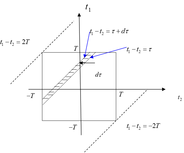
Figure 1.

In the above equation (15), we can think of the process of calculating the area of the square region surrounded by $t_1 = \pm T$ and $t_2 = \pm T$, as shown in Figure 1.

Looking at equation (15), we can see that $t_1-t_2$ is uniformly inserted into the equation, so we can substitute $t_1-t_2=\tau$ and solve the integral expression.

The equation $t_1-t_2 = \tau$ is one of the first-degree functions whose slope is 1. Ultimately, the process of finding the area of the shaded band in Figure 1 by varying $\tau$ from $-2T$ to $2T$ can be seen as the process of solving the integral in equation (15). Therefore, if we denote the area of the shaded band in Figure 1 as $dA$, we can express equation (15) as follows:

\[Equation\ (15)\Rightarrow \frac{1}{2T}\int_{-2T}^{2T}R_{XX}(\tau)\exp(-j\omega \tau) dA\]

Here, $dA$ is given by:

\[dA = (2T-|\tau|)d\tau - \frac{1}{2}(d\tau)^2\]

This is obtained using the difference in the areas of two triangles.

Therefore, by continuing to use equation (16), we have:

\[\frac{E\lbrace X_T(\omega) X_T^*(\omega)\rbrace}{2T}\] \[=\frac{1}{2T}\int_{-2T}^{2T}R_{XX}(\tau)\exp(-j\omega \tau)\left\lbrace(2T-|\tau|)d\tau - \frac{1}{2}d\tau^2\right\rbrace\] \[=\frac{1}{2T}\int_{-2T}^{2T}R_{XX}(\tau)\exp(-j\omega \tau)\left\lbrace(2T-|\tau|) - \frac{1}{2}d\tau\right\rbrace d\tau\] \[=\int_{-2T}^{2T}R_{XX}(\tau)\exp(-j\omega \tau)\left\lbrace \left(1-\frac{|\tau|}{2T}\right) -\frac{1}{4T}d\tau \right\rbrace d\tau\]

Here, if $R_{XX}$ is integrable, as $T$ becomes infinitely large, equation (21) becomes:

\[\int_{-\infty}^{\infty}R_{XX}(\tau) \exp(-j\omega\tau)d\tau\]

Therefore, we can confirm the following relationship:

\[\lim_{T\rightarrow \infty}\frac{E\lbrace |X_T(\omega)|^2\rbrace}{2T} = \int_{-\infty}^{\infty}R_{XX}(\tau)\exp(-j\omega \tau)d\tau\]

As mentioned earlier, the left side of the equation is called the Power Spectral Density $S_{XX}(\omega)$. Therefore,

\[S_{XX}(\omega) = \int_{-\infty}^{\infty}R_{XX}(\tau)\exp(-j\omega \tau)d\tau\]

And, we can also consider:

\[R_{XX}(\tau) = \frac{1}{2\pi}\int_{-\infty}^{\infty}S_{XX}(\omega)\exp(j\omega\tau)d\omega\]

using the inverse Fourier transform.