Prerequisites
To fully understand this post, it is recommended to be familiar with the following content:
Overview
The content that will be covered in this article can be summarized as follows:
- What is a test statistic?
- The meaning of t-value
- Sampling from a population multiple times, calculating their t-values, and directly verifying the distribution
Test Statistic
Before understanding Student’s t-test, it is good to briefly review the concept of test statistic.
In the previous section “Meaning of Sampling and Standard Error”, we learned about populations, parameters, samples, and sample statistics, and finally, we learned that sample statistics are estimates, and the errors in estimation are called standard errors.
Then, what is a test statistic?
A test statistic is a general term for concepts such as t, F, z, and $\chi^2$ that we commonly use when we say “statistical comparison analysis”. Simply put, a test statistic is a statistic calculated from a sample for the purpose of “testing the truth of a statistical hypothesis”.
In other words, the test statistic is a “secondary processed form of sample statistics”, and the process of testing the truth of a statistical hypothesis involves checking whether the value of the test statistic deviates from a predetermined criterion.
Even though this explanation may not be immediately clear, in this article, we will focus on understanding the test statistic through the t-value.
Meaning of t-value: Difference / Uncertainty
When conducting research or investigations, there may be a need to compare the differences between two sample groups. When comparing differences between sample groups, there are various methods that can be used, but the most commonly used measure is the mean.
For example, if you want to confirm the effectiveness of a new drug after developing it, what kind of experiment can you plan?
First, gather as many “healthy” individuals as possible in a clinical setting, then randomly divide them into two groups as randomly as possible, and give placebo medication to one group and the newly developed drug to the other group. Then, you can confirm the effect of the drug.
If you obtain the mean values from each group, can you statistically compare the difference between these two mean values? No, you cannot. These two mean values are sample means, and it should not be forgotten that these sample means always come with errors. In other words, because they are sample means, you need to create a measure of the difference between the two sample groups’ means while considering the errors that occur due to sample means. We have learned about the uncertainty of sample statistics and called it standard error.
Therefore, by dividing the difference by the uncertainty, you can create a statistical measure of the difference.
Statistical measure of sample mean difference: Difference / Uncertainty
Here, the uncertainty refers to the uncertainty of the difference between the means of the two sample groups.
The meaning of t-value is the same as the above-mentioned ‘statistical measure’. In other words, t-value can be interpreted as “this much difference with this much error!”
Let’s mathematically define the t-value.
The difference between the two sample groups can be expressed as $\bar{X_1} - \bar{X_2}$, and the uncertainty mentioned above is related to the difference between the means of the two sample groups, which can be mathematically thought of as the standard error, denoted as $s_{\bar{X_1} - \bar{X_2}}$.
If we give the name ‘t’ to this ‘measure of difference’, we can write it as shown in Figure 1.
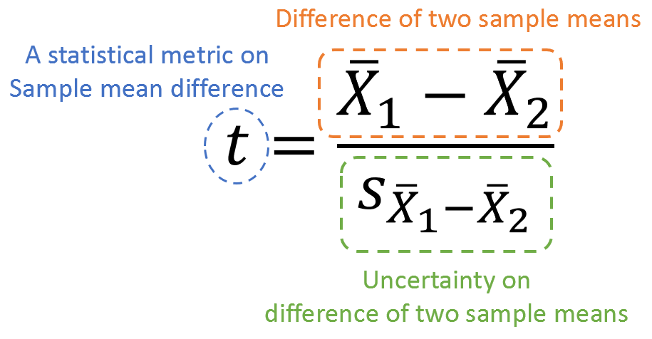
Figure 1. Components and meanings of the t-value
If we further clarify the formula, we can write it as follows.
\[t = \frac{\bar{X_1} - \bar{X_2}}{s_{\bar{X_1} - \bar{X_2}}}\]Let’s further analyze $s_{\bar{X_1} - \bar{X_2}}$ in detail.
\[s_{\bar{X_1} - \bar{X_2}} = \sqrt{Var\left[{\bar{X_1} - \bar{X_2}}\right]}\]And,
\[Var\left[{\bar{X_1} - \bar{X_2}}\right]\] \[= Var[\bar{X_1}] + Var[\bar{X_2}]\] \[= \frac{Var[X_1]}{n_1} + \frac{Var[X_2]}{n_2}\] \[= \frac{s_1^2}{n_1} + \frac{s_2^2}{n_2}\]In going from equation (3) to equation (4), we can view the means of the two groups as independently calculated, so the variance of the difference between the two groups is the sum of the variances of each group. Additionally, in going from equation (4) to equation (5), the calculation is as follows:
From equation (4),
\[\bar{X}_1 = \frac{1}{n_1}\sum_{i=1}^{n_1}X_i\]So,
\[Var[\bar{X}_1] = Var\left[\frac{1}{n_1}\sum_{i=1}^{n_1}X_i\right]\]Here, since $Var[aX]=a^2Var[X]$, we have,
\[= \frac{1}{n_1^2}Var\left[\sum_{i=1}^{n_1}X_i\right]\] \[=\frac{1}{n_1^2}Var\left[X_1+X_2+\cdots+X_{n_1}\right]\]Using the property $Var[X\pm Y] = Var[X] + Var[Y]$, we get,
\[=\frac{1}{n_1^2}\left(Var[X_1]+Var[X_2]+\cdots+Var[X_{n_1}]\right)\]Since $Var[X_1] = Var[X_2] = \cdots = Var[X_n] = s_1^2$, we have,
\[=\frac{1}{n_1^2}\times n_1\times s_1^2 = \frac{s_1^2}{n_1}\]Therefore, by applying the same approach as in equations (7)-(12) to $\bar{X_2}$, we can write:
\[s_{\bar{X_1} - \bar{X_2}} = \sqrt{\frac{s_1^2}{n_1} + \frac{s_2^2}{n_2}}\]Thus, equation (1) can be rewritten as follows:
\[Equation (1) = \frac{\bar{X_1} - \bar{X_2}}{\sqrt{\frac{s_1^2}{n_1} + \frac{s_2^2}{n_2}}}\]Various variations of t-value
The t-value expressed by equation (1) or equation (14) can have different variations depending on the assumptions or settings in the experiment, ultimately centered around the question of “whether to use pooled standard deviation or not?”
Pooled standard deviation (or pooled variance) assumes that the standard deviations of the two groups are equal and uses a single value for the standard deviation of both groups.
When the standard deviations (or variances) of the two sample groups are assumed to be equal (i.e., using pooled standard deviation), we can consider two cases:
First, when the sample size of both groups is the same, i.e., $n_1=n_2=n$, and it is assumed that the variances of the two sample groups are equal, we can write $s_{\bar{X_1} - \bar{X_2}}$ as follows:
\[Equation (1) \Rightarrow \frac{\bar{X_1} - \bar{X_2}}{\sqrt{\frac{s_p^2}{n}+\frac{s_p^2}{n}}}=\frac{\bar{X_1} - \bar{X_2}}{s_p\sqrt{\frac{2}{n}}}\quad\text{where}\quad s_p=\sqrt{\frac{s_1^2+s_2^2}{2}}\]That is, equation (15) is obtained by substituting $s_1$ and $s_2$ with $s_p$ in equation (14), where $s_p$ represents pooled standard deviation.
Second, when the sample sizes of the two groups are different but it is assumed that the variances of the two sample groups are equal, we can write the t-value as follows:
\[Equation (1) \Rightarrow \frac{\bar{X_1} - \bar{X_2}}{\sqrt{\frac{s_p^2}{n_1}+\frac{s_p^2}{n_2}}}= \frac{\bar{X_1} - \bar{X_2}}{s_p\sqrt{\frac{1}{n_1}+\frac{1}{n_2}}}\quad\text{where}\quad s_p=\sqrt{\frac{(n_1-1)s_1^2+(n_2-1)s_2^2}{n_1+n_2-2}}\]The equations (15) and (16) may appear complex, but they are essentially dependent on whether to treat the standard deviation values as pooled or not. Therefore, when applying these formulas in actual research or analysis, one should choose the appropriate formula depending on the specific situation.
Can’t we just divide by the standard deviation?
Looking at equations (14) to (16), they appear to be more complicated compared to the expression in Figure 1, especially with the inclusion of the value of “n” in equations (14) to (16), which makes it difficult to understand the concept of t-value just by looking at these equations, compared to the formula for a normal distribution, which is given as $z=\frac{\bar{X}-\mu}{\sigma}$.
Why is “n” included in the formula for t-value?
The reason can be better understood by looking at Figure 2 below.
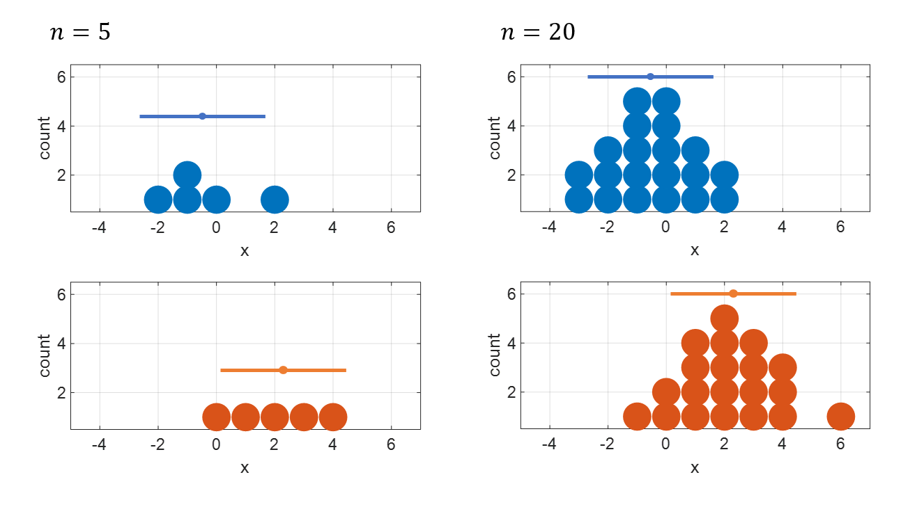
Figure 2. The larger the sample size, the more accurately the mean values of the two samples can be calculated.
In other words, as the sample size increases, the standard error of the sample mean decreases.
From Figure 2, it can be seen that as the sample size (i.e., “n”) increases, the mean values of the two samples can be calculated with more confidence. When considering the comparison between the two groups on the left and the two groups on the right in Figure 2, this concept becomes easier to understand.
The expression “with more confidence” may seem non-mathematical, but to put it in more mathematical terms, as the sample size increases, the standard error of the sample mean decreases, allowing for more confident calculations.
How is the threshold for a sufficiently large t-value determined?
As mentioned earlier in the “Test Statistic” section of this article, the t-value, which is one of the test statistics, is no different from a processed version of the sample statistics.
As demonstrated in the article on the meaning of sample and standard error, by repeatedly extracting two random sample groups from a population with a size of 150 and n=6 and calculating the t-value, the distribution of t-values can be observed. Let’s take a look at this process repeated 100 times.
Figure 3. Plot of t-values obtained from extracting 100 pairs of sample groups with n=6 from a single population
From Figure 3, it can be observed that when extracting two sample groups from a single population and calculating the t-value, in many cases, the t-value is calculated to be close to 0. However, sometimes t-values with values such as 2 or 3 are obtained, despite being calculated from a single population.
In other words, when a sufficiently large t-value is calculated from two sample groups, it indicates the following:
Assuming that two sample groups came from the same population, the probability of obtaining such a large t-value is very low. Therefore, we can say that the probability of these two sample groups coming from the same population is also very low.
In fact, there are almost an infinite number of possibilities for sample extraction processes like the one shown in Figure 3, not just 100. For example, if the population size is 150 and two sample groups of n=6 are selected, the number of possible cases is:
\[_{150}C_{12} = 172,420,656,389,440,550\notag\]Since it is impossible to perform sample extraction for numerous cases like this, the distribution of t-values has been mathematically calculated and formalized as the t-distribution (solid line in Figure 3).
Reference
- Primer of biostatistics 6th edition, Stanton A Glantz, McGraw-Hill Medical Publishing Division