Prerequisites
To understand this post, it is recommended that you have knowledge of the following:
- The meaning of the existence of imaginary numbers
- The meaning of the natural constant e
- The geometric meaning of Euler’s formula
- The geometric meaning of eigenvalues and eigenvectors
Eigenvalues and eigenvectors of rotation matrices
\[A=\begin{bmatrix}\cos(\theta) && -\sin(\theta) \\ \sin(\theta) && \cos(\theta)\end{bmatrix}\]For example, applying the matrix that rotates counterclockwise by 90 degrees results in the following linear transformation:
\[\begin{bmatrix} \cos(\pi/2) & -\sin(\pi/2) \\ \sin(\pi/2) & \cos(\pi/2) \end{bmatrix}\]
Figure 1. Visualization of a linear transformation that rotates counterclockwise
The key point from the meaning of eigenvalues and eigenvectors is as follows:
"Then, how much did the magnitude change?"
Then, the question arises: where are the vectors that only change in magnitude and not in direction when the rotation transformation is applied?
Calculation of eigenvalues and eigenvectors
To understand the meaning of the eigenvalues and eigenvectors of rotation matrices, let’s try to calculate them directly.
Calculation of Eigenvalues
\[A\vec{x}=\lambda\vec{x}\] \[=\begin{bmatrix}\cos(\theta) && -\sin(\theta) \\ \sin(\theta) && \cos(\theta)\end{bmatrix}\vec{x} = \lambda\vec{x}\]Here, $\vec{x}$ can also be thought of as decomposed into $I\vec{x}$.
Here, $I$ is an identity matrix as follows.
\[I=\begin{bmatrix}1 && 0\\0 && 1\end{bmatrix}\] \[\Rightarrow \begin{bmatrix}\cos(\theta) && -\sin(\theta) \\ \sin(\theta) && \cos(\theta)\end{bmatrix}\vec{x} = \lambda I\vec{x}\]Moving the right-hand side to the left-hand side,
\[\Rightarrow (A-\lambda I)\vec{x} = \begin{bmatrix}\cos(\theta)-\lambda && -\sin(\theta) \\ \sin(\theta) && \cos(\theta)-\lambda\end{bmatrix}\vec{x}=\vec{0}\]In order for $\vec{x}$ not to be a zero vector, $(A-\lambda I)$ should not have an inverse, so the determinant of $(A-\lambda I)$ should be 0.
\[det(A-\lambda I)=(\cos(\theta)-\lambda)^2+\sin^2(\theta) = 0\] \[=\cos^2(\theta) - 2\lambda\cos(\theta) + \lambda^2 + \sin^2(\theta)=0\]Here, $\cos^2(\theta) + \sin^2(\theta) = 1$, so
\[\Rightarrow \lambda^2 -2\lambda\cos(\theta) + 1 = 0\]Applying the quadratic formula, we can calculate $\lambda$ as follows.
\[\lambda = \cos(\theta) \pm\sqrt{\cos^2(\theta)-1}\] \[=\cos(\theta)\pm\sqrt{-\sin^2(\theta)}\] \[=\cos(\theta) \pm i\sin(\theta)\]Here, $i=\sqrt{-1}$.
Now, let’s calculate the eigenvector corresponding to each eigenvalue.
1. Eigenvector for the case of $\lambda=\cos(\theta)+i\sin(\theta)$
In the case of $\lambda = \cos(\theta) + i\sin(\theta)$,
\[\begin{bmatrix}\cos(\theta) && -\sin(\theta) \\ \sin(\theta) && \cos(\theta)\end{bmatrix}\vec{x} = (\cos(\theta) +i\sin(\theta))\vec{x}\]must be satisfied.
If we move the right-hand side to the left-hand side,
\[\Rightarrow \begin{bmatrix}-i\sin(\theta) && -\sin(\theta) \\ \sin(\theta) && -i\sin(\theta)\end{bmatrix}\vec{x}=0\]then we can say that the product of the matrix and the vector above is equivalent to solving the following system of linear equations.
If we define vector $\vec{x} = \begin{bmatrix}x_1, x_2\end{bmatrix}^T$,
\[\begin{cases} -i\sin(\theta) x_1 - \sin(\theta)x_2 =0 \\ \sin(\theta)x_1 - i\sin(\theta)x_2 =0 \end{cases}\]and if we divide all equations by $\sin(\theta)$ here,
\[\begin{cases} -i x_1 - x_2 =0 \\ x_1 - i x_2 =0 \end{cases}\]so,
\[\vec{x}=\begin{bmatrix}i\\1\end{bmatrix}\]for this case.
2. Eigenvector for $\lambda=\cos(\theta)-i\sin(\theta)$
If we compute the eigenvector in a similar way as in the previous section,
the eigenvector for the case of $\lambda=\cos(\theta)-i\sin(\theta)$ is
\[\vec{x}=\begin{bmatrix}-i\\1\end{bmatrix}\]Another perspective on eigenvalues and eigenvectors
Once again, in the previous article on the geometric interpretation of eigenvalues and eigenvectors, we discussed the following:
"So, how much has the magnitude changed?"
That is, the focus of the previous perspective can be seen as the process of finding eigenvalues and eigenvectors for a given linear transformation.
However, let’s think about it from another perspective. If we know the appropriate eigenvalues and eigenvectors, the meaning of the eigenvalue for a given eigenvector is as follows:
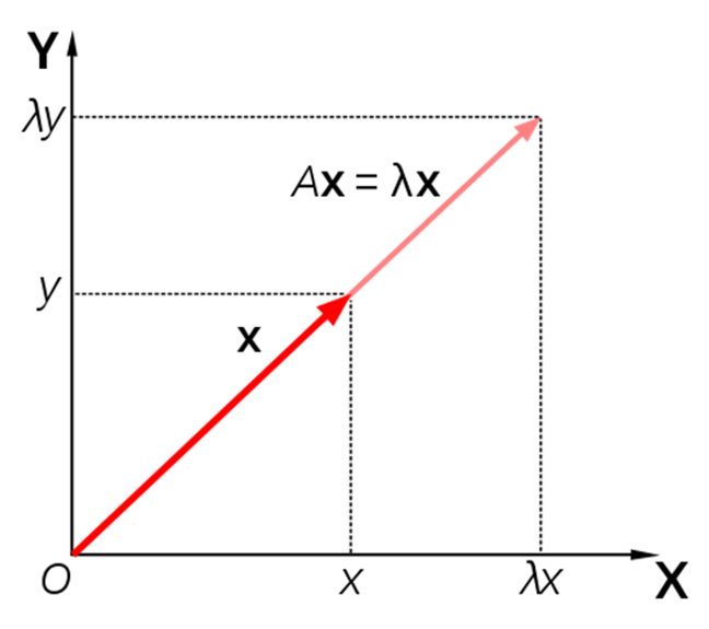
Figure 2. When a linear transformation is applied to an eigenvector, it is just a scalar multiple of the eigenvalue.
What is scalar multiplication?
Scalar multiplication is a fundamental property that a vector must have, as discussed in the basic vector operations (scalar multiplication, addition) article.
However, its fundamental meaning lies in ‘multiplication’.
As mentioned in the meaning of the existence of imaginary numbers article, multiplication has directionality.
Multiplying by a negative number means a transformation in the opposite direction, and multiplying by a complex number means ‘rotation’.
Figure 3. Geometric interpretation of multiplying by a complex number (in this case, a purely imaginary number)
Also, in the geometric interpretation of Euler’s formula, we learned that the complex number
\[\exp(i\theta) = \cos(\theta) + i \sin(\theta)\]represents rotating the number 1 on the complex plane by an angle of $\theta$ radians. As n increases in the animation in Figure 4 of the post, the point transformed by $\cos(\theta)$ and $\sin(\theta)$ on the complex plane moves. For more detailed information, refer to the geometric interpretation of Euler’s formula.
In the end, the meaning of a complex eigenvalue lies in “rotating a vector through complex multiplication” rather than changing the length of the vector.
Visualization of Complex Eigenvectors
On the other hand, how should we think about the complex eigenvectors we obtained for the rotation matrix?
The reason why it is difficult to visualize or understand complex eigenvectors is that complex numbers themselves are already 2-dimensional.
To elaborate a bit more, a complex number has two numbers that go into its “real part” and “imaginary part.”
Therefore, a 2-dimensional complex vector has a total of four real numbers, and since we do not have a way to understand the world in four dimensions, there is no precise way to represent a 2-dimensional complex vector.
However, I would like to visualize the two complex vectors we obtained in my own way.
The complex vectors we obtained were as follows:
\[v_1 = \begin{bmatrix} i \\ 1 \end{bmatrix}\] \[v_2 = \begin{bmatrix} -i \\ 1 \end{bmatrix}\]We can visualize each complex vector as follows:
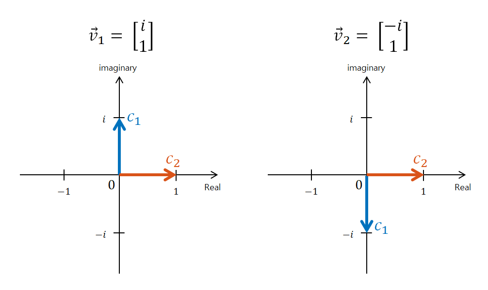
Figure 5. Visualization of complex vectors $v_1$ and $v_2$. $c_1$ and $c_2$ within the figure represent the first and second elements of each vector, respectively.
The most noteworthy part in the above figure is that although $\vec{v}_1$ and $\vec{v}_2$ are represented by two arrows, we should consider these two arrows as one vector.
To reiterate what is important, it is the representation of a complex vector with two arrows.
Interaction between rotation matrix and eigenvectors
Now let’s think again about the following phrase:
What does it mean to scale the complex vectors $\vec{v}_1$ and $\vec{v}_2$ represented in Figure 5 by the corresponding eigenvalues?
Since the eigenvalues are $\exp(i\theta)$ and $\exp(-i\theta)$, they represent a rotation of $\theta$ radians clockwise or counterclockwise, respectively.
In other words, scaling the complex vectors $\vec{v}_1$ and $\vec{v}_2$ by the corresponding eigenvalues means rotating the eigenvectors counterclockwise or clockwise by $\theta$ radians, respectively.
Let’s visually explore the interaction between the rotation matrix and eigenvectors for two different eigenvalues by moving the slider in Figures 6 and 7.
\[A=\begin{bmatrix}\cos(\theta) && -\sin(\theta) \\ \sin(\theta) && \cos(\theta)\end{bmatrix}\]
Figure 6. Interaction between rotation matrix and eigenvectors for $\lambda_1 = \exp(i\theta)$. The white arc in the top right corner corresponds to the rotation angle.
Figure 7. Interaction between rotation matrix and eigenvectors for $\lambda_2 = \exp(-i\theta)$. The white arc in the top right corner corresponds to the rotation angle.
Again, the results of Figures 6 and 7 ultimately show that scaling a vector can be represented in the realm of complex numbers. However, it should be noted that this discussion is limited to the special cases of eigenvalues and eigenvectors.
References
- Visualizing the eigenvectors of a rotation / Twisted Oak Studios