So far, we have learned about what vectors are and how to interprete matrix-vector multiplication. In short, a vector is a collection of elements that follow scalar multiplication and addition rules, and the set of these elements with defined operations is called a vector space. The elements that follow these scalar multiplication and addition rules are said to have “linearity.” A matrix is an operator that transforms one vector into another, and matrix-vector multiplication can be seen as a way to combine the column vectors of a matrix by a linear combination.
In this session, we will explore the function and role of row vectors and how they relate to the geometric meaning of vector dot products and projections between vectors.
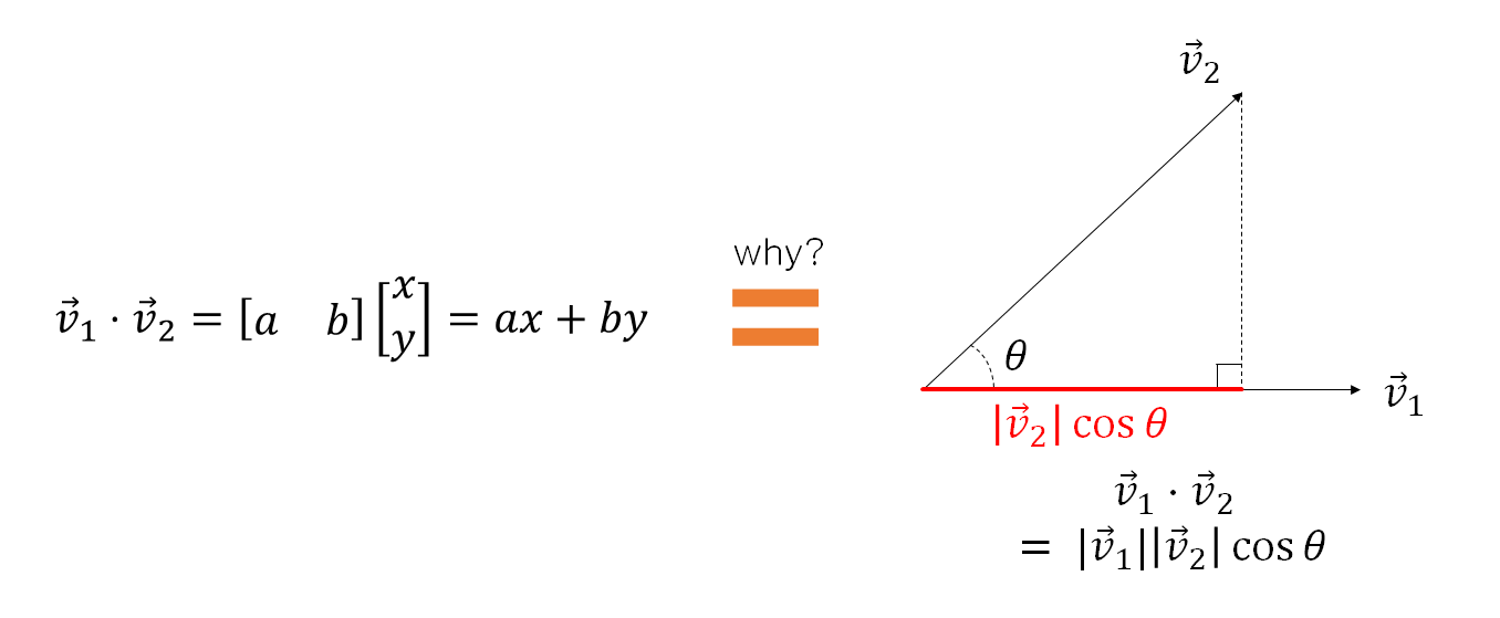
Figure 1. What is the function and role of row vectors, and how is it related to the geometric meaning of vector dot products and projections between vectors?
Function and Role of Row Vectors
When considering matrix-matrix or matrix-vector multiplication, the most basic way to interpret matrix multiplication is to multiply each element of the left matrix with its corresponding element of the right matrix and then sum them up in order.
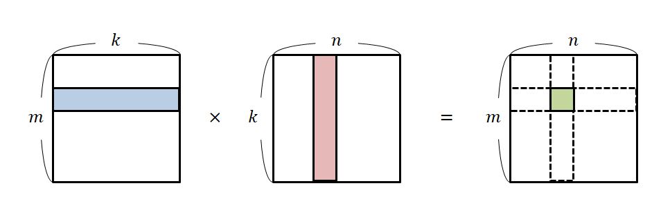
Figure 2. The most basic interpretation of matrix multiplication
In the previous article on a new understanding of matrix multiplication, we mentioned that this interpretation can be understood as the dot product between row vectors and column vectors. However, let’s assume that we do not know the term “dot product” or its calculation method and focus solely on matrix multiplication. In this case, let’s explore what happens between row vectors and column vectors.
When we talk about “vectors,” we typically refer to column vectors as the “common” vectors in mathematics. This is a mathematical convention that we have set as a standard. In other words, we conventionally view column vectors as the objects that undergo transformations.
On the other hand, a row vector is a function on a column vector. In other words, while a column vector is the “subject of change,” a row vector is the “agent of change” that brings about the transformation.
For instance, let us consider the following multiplication of a row vector $[2, 1]$ and a column vector $[3, -4]^T$:
\[\begin{bmatrix}2 & 1\end{bmatrix}\begin{bmatrix}3\\-4\end{bmatrix} = 2\cdot 3 + 1\cdot(-4) = 6-4 = 2\]Alternatively, we can represent this as a function notation:
\[\begin{bmatrix}2 & 1\end{bmatrix}\left(\begin{bmatrix}3\\-4\end{bmatrix}\right) = 2\]In other words, a row vector is a function $f:V\rightarrow\Bbb{R}$ that takes in a column vector as input and outputs a scalar value.
Visualization of Row Vectors
So far, we have mentioned that a row vector is a function that takes in a column vector as input. Can we visualize a row vector as a function?
To visualize a function, we represent the output $f(x)$ of a function at any given input $x$ as a point on the coordinate plane.
For instance, to visualize $y=x^2$, we plot all values of $y=f(x)=x^2$ for a range of $x$ that is easy to plot, say, $-2\leq x \leq 2$.
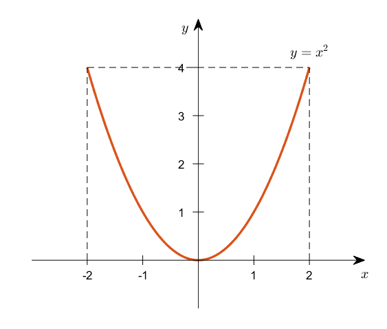
Figure 3. Visualization of the function $y=x^2$ for the range of $-2\leq x \leq 2$
Similarly, to visualize the row vector $\begin{bmatrix}2 & 1\end{bmatrix}$, we can plot the output values on a coordinate plane for an arbitrary vector $\begin{bmatrix}x & y \end{bmatrix}^T$.
\[\begin{bmatrix}2 & 1 \end{bmatrix}\left(\begin{bmatrix}x \\ y \end{bmatrix}\right) = 2x+ y\]Since a row vector takes in a column vector and outputs a scalar value, we can display several outputs on a single $x, y$ plane.
For example, we can represent all pairs of $x$ and $y$ that satisfy $2x+y=1$ on the line $y=-2x+1$.
Using the concept of contour lines, we can represent multiple scalar output values at once.
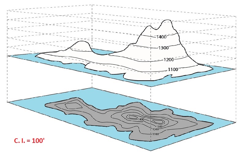
Figure 4. An example of a contour map. Contour lines connect points of equal height with curved lines.
Image source
As the name implies, a contour map is a map that connects points of the same height with a single line. Here, let’s connect pairs of $x, y$ values that have the same scalar output value to form a single line.
In other words, using this contour map, we can easily visualize the output values of an arbitrary vector $\vec{v}$ that passed through the function $\begin{bmatrix} 2 & 1\end{bmatrix}$.
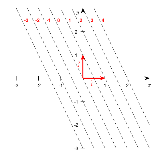
Figure 5. Visualization of output values of a function through a row vector.
Looking at Figure 5, we can see that the output values of $2x+y$ are represented by a single line that corresponds to values from -3 to 4 for $x$ and $y$ pairs.
If we represent some of these pairs as vector arrows, we can see examples of the input column vectors that produce each output value in Figure 6.
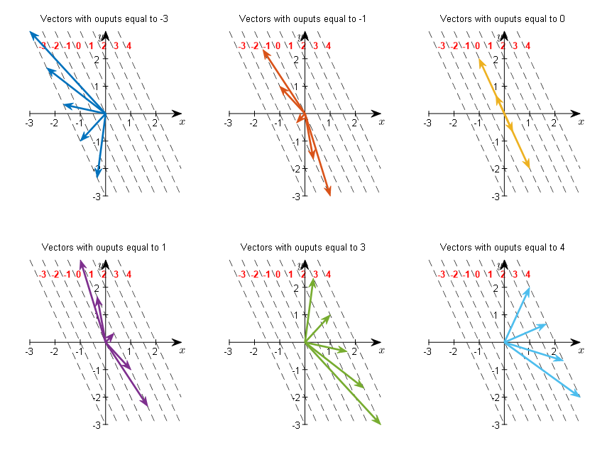
Figure 6. Examples of column vectors that produce different output values for the row vector function.
For instance, looking at the vectors with an output value of -3 at the top left of Figure 6, we can see that they form a set of vectors that have endpoints on the dotted line $2x+y=-3$.
Inner Product between Row Vectors and Vectors
Now let’s think about the geometric meaning of the inner product between two vectors $\vec{v}_1$ and $\vec{v}_2$, as we can see in the right side of Figure 1. If the angle between the two vectors is $\theta$, we know that the inner product of the vectors is calculated as follows.
\[\vec{v}_1\cdot\vec{v}_2 = |\vec{v}_1||\vec{v}_2|\cos\theta\]From this, we can also see that $|\vec{v}_2|\cos\theta$ is the projection of $\vec{v}_2$ onto the direction of $\vec{v}_1$.
Let’s consider the case where the output scalar value is 4 among the various subplots in Figure 6. If we think of an arbitrary vector that produces an output scalar value of 4 and draw it, it will look like the following.
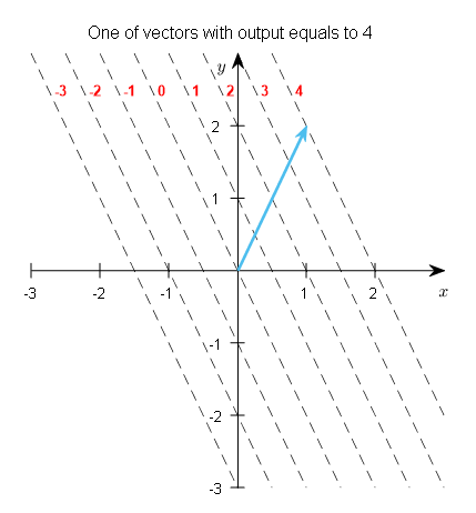
Figure 7. Let's think of an arbitrary vector that produces an output scalar value of 4.
What does it mean for the output scalar value to be 4? Let’s draw the row vector $[2, 1]$ and think about the distance to the point $2x+y=4$.
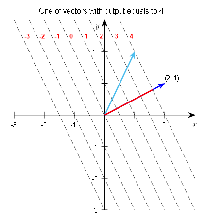
Figure 8. The row vector $[2, 1]$ (dark blue) and the distance to $2x+y=4$ (red).
If we think about it, the dotted line corresponding to $2x+y=c$ is perpendicular to all row vectors $[2, 1]$. This is because the row vectors serve as the normal vectors for the functions represented by the dotted lines.
Therefore, we can obtain the length represented by the red line in Figure 8 by calculating the height of the right triangle, as shown in Figure 9.
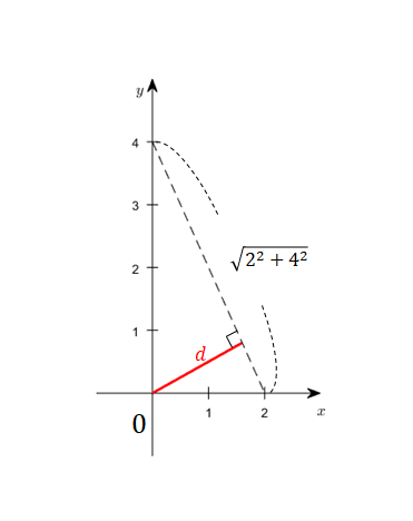
Figure 9. The length of $d$ can be calculated using the method for finding the area of a right triangle.
That is,
\[4\times 2 = d\times \sqrt{20}\]so,
\[d= \frac{8}{\sqrt{20}}=\frac{4}{\sqrt{5}}\]Here, the length of the row vector $[2,1]$ is $\sqrt{5}$. Multiplying this length by $d$ gives
\[d\times\sqrt{5} = \frac{4}{\sqrt{5}} * \sqrt{5} = 4\]This shows that the length of the projection of the column vector onto the row vector multiplied by the length of the row vector is equal to the dot product.
In fact, as shown in Figure 7, when calculating the dot product of two vectors, any vector on the dashed line $2x+y=4$ will yield a dot product of 4 with the row vector $[2,1]$.
Geometrically, this means that the length of the projection of the column vector is used in the dot product calculation.
Row Vectors and Row Spaces
Like column vectors, row vectors satisfy the definition of vectors and exhibit linearity, so they can be thought of as general vectors.
But why is it important to determine whether row vectors exhibit linearity? It’s because if a row vector, which represents a ‘function’ rather than ‘data,’ exhibits linearity, then all methods that are known to apply to general vectors can also be applied.
First, as with column vectors, vector addition is defined for row vectors.
A row vector as a function is represented by $f$, and for any two column vectors $\vec{v}$ and $\vec{w}$, the following holds:
\[f(\vec{v}+\vec{w}) = f(\vec{v}) + f(\vec{w})\]For example, it can be easily seen that the left and right sides of the following equation are equal:
\[\begin{bmatrix}2 & 1\end{bmatrix}\left(\begin{bmatrix}3\\-4\end{bmatrix} + \begin{bmatrix}1\\2\end{bmatrix}\right) = \begin{bmatrix}2 & 1\end{bmatrix}\left(\begin{bmatrix}3\\-4\end{bmatrix}\right) + \begin{bmatrix}2 & 1\end{bmatrix}\left(\begin{bmatrix}1\\2\end{bmatrix}\right)\]Furthermore, scalar multiplication is defined for row vectors.
For any scalar $n$, the following holds:
\[f(n\vec{w}) = nf(\vec{w})\]For example, it can be easily seen that the left and right sides of the following equation are equal:
\[\begin{bmatrix}2 & 1\end{bmatrix}\left(2\begin{bmatrix}3 \\ -4\end{bmatrix}\right)= 2\begin{bmatrix}2 & 1\end{bmatrix}\left(\begin{bmatrix}3 \\ -4\end{bmatrix}\right)\]To summarize, a row vector has the following functions and properties:
- It is a function that takes a column vector as input and outputs a scalar (i.e. a number).
- It is a linear operator.
- In other words, the sum of two vectors as input and the sum of their function outputs are the same.
- Also, because it is a linear operator, multiplying the input by a constant and multiplying the output by the same constant yield the same result.
The Geometric Meaning of Row Vectors as Linear Functions
Scalar Multiplication of Row Vectors
In Figure 6, we used contour lines to represent the scalar output values obtained when an input column vector is applied to a row vector.
If we think about this picture again, we can consider the way we get the scalar value output after operating on a given row vector with a given column vector as the number of contour lines that the column vector passes through.
Therefore, we can see that if the length of the row vector increases, the contour lines become narrower.
Conversely, if the length of the row vector decreases, the contour lines become wider.
Figure 10. Visualization corresponding to row vectors of varying sizes that become larger or smaller with various scalar multiples
Addition of Row Vectors
Furthermore, the addition of row vectors means that two different contour lines can be combined to create a new contour line.
At this point, the new contour line is formed perpendicular to the new row vector obtained by adding the row vectors corresponding to the two different contour lines.
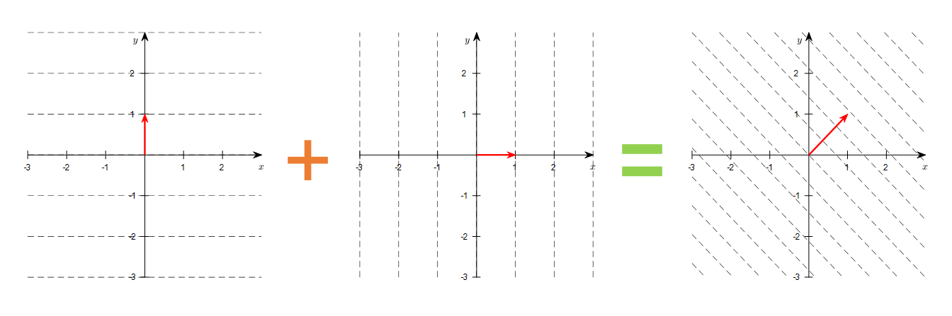
Figure 11. Visualization of the contour line corresponding to the new row vector obtained by adding two row vectors
Row space is the dual space of the column space.
When defining vectors, we said that we define vectors as those that are defined with scalar multiplication and addition between vectors, and that these vectors form a vector space. Therefore, we can also consider row vectors, which can be thought of as linear functions[^1] for row vectors, as general vectors.
The set of row vectors consisting of defined addition and multiplication laws is called the row space. Although we have been calling row vectors “row vectors” so far, we can think of them as new concepts of vectors by using strict criteria like this.
The row space is called the dual space because it corresponds to the column space, and the strict definition of the dual space is as follows:
| DEFINITION Dual Space |
|---|
| The set of linear functionals of a vector space $V$ is called the dual space $V^*$ of $V$. $$V^*=\left\lbrace f:V\rightarrow \Bbb{R} | f(c\vec{a}+\vec{b})\text{ for all }\vec{a},\vec{b}\in V\right\rbrace$$ |
The concept of dual space is important because in cases where it is difficult to solve a problem in the original vector space, there are cases where the problem can be easily solved in the corresponding dual space.
For example, the transformation between time and frequency in linear algebraic interpretation of linear regression or Fourier transform both utilize the concept of duality.