Geoffrey Hinton mentioned in an interview with Andrew Ng that if he had to name the most proud achievement in his career as a researcher, it would be the research results using RBM.

Hinton’s contribution using RBM demonstrated how important it is to initialize deep neural networks. This is because the success or failure of how effectively deep neural networks are learned depends on how they are initialized.

RBM is a generative model that can probabilistically obtain latent factors of data. In this post, we will explore how RBM works.

Prerequisites

To understand RBM well, it is recommended that you have a good understanding of the following:

• Maximum Likelihood Estimation
• Gradient descent
• Rejection Sampling
• Monte Carlo Markov Chain

• If we know the probability distribution…

The Restricted Boltzmann Machine (RBM) is a generative model, and it has a slightly different goal from deterministic models such as ANN, DNN, CNN, and RNN.

If the goal of deterministic models is to reduce errors by minimizing the difference between the target and the hypothesis, the goal of generative models is to model the probability density function.

What does it mean to know the probability density function (PDF) accurately?

Suppose there is a machine that draws faces. Faces are composed of various elements, such as the nose. The nose is also composed of various possible shapes. Suppose we assume that only circular, triangular, and rectangular noses exist in the world. If we can know the probability density function for these three shapes of noses, that is, we investigated the shape of the nose in all faces in the world and drew a histogram, …

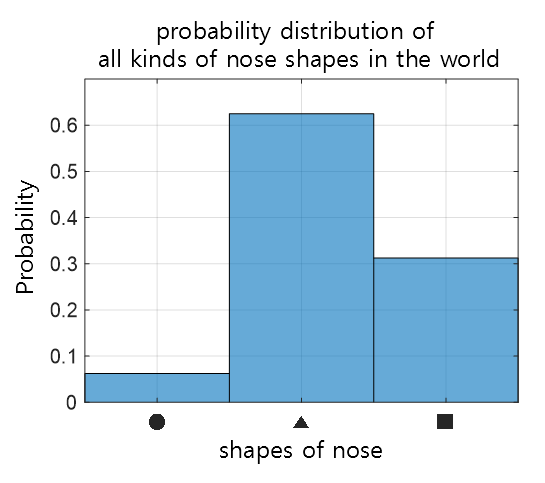
Figure 1. Probabilistic distribution of the shapes of nose

Looking at the image above, we can see that a triangular-shaped nose (▲) is the most common nose shape in the world.

If a machine that draws faces knows about this probability distribution, it is more likely to draw a triangular-shaped nose when drawing a nose.

If we can accurately know the probability of an event occurring for all possible cases, we can reasonably generate an event (in this case, a whole face) composed of various events.

In fact, faces generated using Generative Adversarial Networks (GANs), which are currently popular generative models, can be seen in the following figure.

Figure 2. Evolution of faces generated using GAN
Source

The process of generating a result (in this case, a face) using a probability density function is called sampling.

In summary, the goal of a generative model is to learn the probability distribution accurately and generate good samples through sampling.

Machine Design for Learning Probability Density Functions

Boltzmann Machine

The Boltzmann Machine can be said to have been created to learn probability distributions (more precisely, probability mass functions or probability density functions).

What the Boltzmann Machine assumes is, “If we can include not only what we see but also elements that are not visible in the learning process, can’t we know the probability distribution more accurately?”.

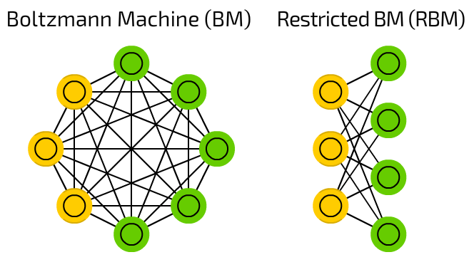
Figure 3. Boltzmann Machine and Restricted Boltzmann Machine
Source of Image

What is shown on the left in Figure 3 is the Boltzmann Machine, and what is shown on the right is the Restricted Boltzmann Machine.

First, let’s explain the Boltzmann Machine. The circular shapes represent states for possible events.

For example, suppose this Boltzmann Machine was created to learn the probability density function of face shapes, and each circle represents a state for a specific part of the face.

One of the circles might represent the nose, and states 0, 1, and 2 might represent the nose in the form of a circle, triangle, and square, respectively.

Another notable point in the Boltzmann Machine is the yellow and green features, each of which represents the presence of hidden units and visible units, respectively.

The hidden unit implies the existence of some feature that we cannot see, and assumes that if we can learn even these invisible factors, we can learn a more accurate probability distribution.

Restricted Boltzmann Machine

So what is the Restricted Boltzmann Machine (RBM), which is our topic of interest?

As shown on the right-hand side of Figure 3, the RBM is derived from the Boltzmann Machine and has a structure in which there are no internal connections between visible units and hidden units, but only connections between visible units and hidden units remain.

There are several practical reasons for constructing RBMs in this way related to various probability calculations.

First of all, the absence of internal connections between nodes in the visible and hidden layers assumes independence between events, making it easy to express joint probability distributions.

In addition, by only connecting the visible layer and the hidden layer, RBMs can calculate ‘conditional probabilities’ that enable calculation of hidden layer data given visible layer data or visible layer data given hidden layer data.

In other words, $p(h,v)$ is difficult to calculate, while $p(h|v)$ or $p(v|h)$ is relatively easy to calculate.

In summary, RBMs were constructed to make Boltzmann Machine calculations easier, as they became too complex.

One unique feature of RBMs created by constructing a form similar to FFNNs (Feed-Forward Neural Networks) is that they learn in a manner similar to FFNNs.

As I will explain later, the operation of RBMs determines the state of the hidden units through forward propagation similar to FFNNs and then determines the state of the visible units again by back-propagation from the hidden units’ state.

Structure and Characteristics of RBM

As mentioned earlier, learning in an RBM involves acquiring a probability distribution. So, how can we mathematically express that an RBM has learned well?

To understand this, let’s take a closer look at the structure of RBMs.

Structure of RBMs

Figure 4. A more detailed structure of RBMs
Source of the figure

As we can see from the structure of an RBM, it consists of a visible layer, a hidden layer, and a weight matrix that connects the two layers. In addition, there are bias terms included in both the visible and hidden layers.

Here is a brief explanation of each component:

• Visible layer: Where input data is fed into. Each input data can have multiple states. It will be denoted by $v$.
• Hidden layer: Where hidden data is sampled. Each hidden data can have multiple states. It will be denoted by $h$.
• Weight matrix: The device that connects the visible layer and hidden layer. It is derived from the original Boltzmann Machine. It will be denoted by $W$.
• Bias for visible layer: The part that sets the inherent property of the input data. As we will discuss later, if a visible unit is almost always 1, a higher bias for that unit is better. It will be denoted by $b$.
• Bias for hidden layer: The part that sets the inherent property of hidden data. It plays a similar role to the bias for the visible layer. It will be denoted by $c$.

Note that all of the aforementioned $v$, $h$, $b$, $c$ are vectors and $W$ is a matrix.

When there are $d$ nodes in the visible layer and $n$ nodes in the hidden layer, the dimensions are as follows:

Let’s continue to explore how to express that a Restricted Boltzmann Machine (RBM) with this structure is “learning well.”

Energy: A Numerical Measure of Configuration

To numerically evaluate whether an RBM is learning well, we need to define a cost function as we would with other models.

The cost function for an RBM is uniquely defined using a concept called “energy,” which is borrowed from physics.

If we call the energy of a particular state $x$ as $E(x)$, then $E(x)$ is a value that corresponds to that state (configuration).

In other words, $E(x)$ can be thought of as indicating the distribution of events in state $x$, and thus it can be connected to a probability distribution.

If we calculate the probability of obtaining the desired energy value for state $x$ among all possible energy functions from a multinomial distribution, we can calculate the probability value for a specific state $x$ as follows:

However, in RBM, we can determine the energy based on the states of visible units $v$ and hidden units $h$, and ultimately we can determine the probability distribution of visible units as the energy due to visible units $v$ is observable. Thus, we can determine the probability distribution of visible units as follows:

Introducing the concept of hidden units, Equation (4) becomes complex like Equation (6), so let us substitute it to make Equation (6) similar to Equation (4).

Let’s name $F(\cdot)$ the Free Energy.

Meanwhile, in RBM, energy is defined as follows:

Here, the $’$ sign represents transpose. In other words, $b’v$ means the dot product of the $b$ vector and the $v$ vector.

Did RBM define energy as in Equation (11)? This can be confirmed through the explanation of $b, c, W$, especially that $b$ and $c$ set the inherent characteristics of the visible layer and the hidden layer, respectively.

In other words, these bias terms need to be transformed according to the characteristics of the given data. These bias terms will be set to increase in value depending on how often a certain visible unit or hidden unit is in the “ON” state. If a certain visible unit is almost always 1, then the bias of that unit will be high, and as a result, the energy value in Equation (11) will decrease. Low energy means a stable state.

RBM with two states

In many RBM studies, Bernoulli RBM is used, which is an RBM that has visible or hidden units with only two states, 0 or 1. We will later learn more about how we can determine if RBM is learning well using the concept of energy. To develop the learning process of RBM using the equation (11) for Energy, we can use the equation (9) for Free Energy because the equation for Energy can become very complex. Therefore, let’s first expand the formula for Free Energy.

Since $exp(b’v)$ does not contain terms related to $h$, it can be brought out of the summation:

Since $\log(\exp(x))$ is equal to $x$, we have:

Here, $h\in{0, 1}$, so we can simplify it further:

Here, $W_i$ represents a row vector obtained from the $i$th row of $W$.

Moreover, RBM’s unique structure allows us to sample hidden layer data using visible layer data and vice versa. Therefore, we can calculate the conditional probability of sampling hidden layer data when visible layer data is given (or vice versa).

In this context, let’s calculate the probability $p(h_i=1|v)$ that the $i$-th hidden layer unit among the $n$ hidden layer units will be sampled as 1, given the visible layer $v$.

In Bernoulli RBM, where $h\in\lbrace 0, 1\rbrace$, we have:

Here, $\sigma(\cdot)$ is the sigmoid function.

Similarly,

where $W_j’$ represents a row vector obtained from the $j$-th column of the matrix $W$.

Learning Process of RBM

Overview of RBM Learning Process

Now, most of the basic equations needed for RBM learning have been developed.

So, what does it mean to train an RBM?

We can say that the goal of RBM is to learn a probability distribution, and the process of RBM learning can be indirectly confirmed through sampling.

If RBM has learned a given data well, the data obtained through sampling in the visible layer should be almost the same as the original data.

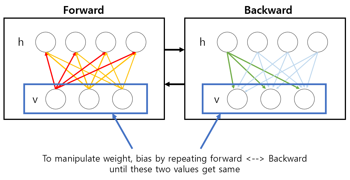
Figure 4. The meaning of training RBM: the sampled visible layer values become the same as the original visible layer values.

Let’s derive this process mathematically.

RBM Learning with Gradient Descent

The fact that the data obtained through sampling in the visible layer has almost the same shape as the original data is not an arbitrary learning goal if RBM’s parameters ($b, c, W$) are well learned.

Let’s mathematically confirm this.

If the parameters of RBM are well learned, then the product of all the likelihoods obtained through the current data will be maximized.

(In case this sentence is not clear, it is recommended to study maximum likelihood estimation before continuing!)

In other words, to learn RBM’s parameters well, the height of the probability density function obtained through the current data using the probability function defined for the visible layer in equation (8) must be maximized by multiplying all the heights of the probability density functions obtained through the data.

However, the learning process means that the learning is incomplete, so to maximize the likelihood (i.e., the height of the probability density function obtained through all the data), we can use the Gradient ascent method. However, when we usually train a model, we perform Gradient descent, so let’s minimize the negative likelihood by multiplying it by -1. Therefore, we will use the Gradient Descent method.

Furthermore, it is generally common to use log-likelihood rather than likelihood directly, so let’s calculate the equation to minimize the negative log-likelihood. Let’s refer to RBM parameters as $\theta$. Now, from equation (8), the negative log-likelihood can be calculated as follows:

Here, $\tilde v$ refers to a sample of visible units generated by the RBM model.

Based on the definition of expected value,

Since it is impossible to actually calculate expected value, we can consider the data of visible layers obtained through sampling, denoted as $\mathcal{N}$, as follows:

In the last equation, we can see that the difference between the free energy of the original visible layer data $v$ and the free energy of the visible layer data $\tilde{v}$ obtained through sampling is used as the loss in RBM.

In other words, a low loss in RBM means that the visible layer data obtained through sampling has a shape that is very similar to the original data, confirming this fact once again.

In the end, learning for RBMs means reducing Contrastive Divergence (CD).

CD refers to the difference between the originally given visible layer data and the obtained visible layer data when the node values of the hidden layer are sampled and then the data in the visible layer are predicted again.

If the weight matrix and the hidden layer bias are well learned, the hidden units can be sampled well, and therefore the re-obtained visible layer data will match the original data.

Here, Professor Hinton experimentally confirmed that RBM learning does not have much difficulty even if the visible layer data is sampled only once to calculate the loss.

Therefore, the loss can be thought of as the difference between the free energy of the visible layer obtained from the original data and the free energy of the visible layer obtained from the generated data, which indicates that learning is better when this difference is small. The loss can be expressed as follows:

Sampling Process

So how can we sample data from the visible or hidden layer?

Gibbs sampling is one of the methods of Markov Chain Monte Carlo. Since it uses the characteristic of Markov Chain, it can be considered as Gibbs Sampling for RBM sampling. Although the name sounds complicated and fancy, it is simply an Accept/Reject through likelihood comparison.

The fact that $\vec{v}$ and $\vec{h}$ in RBM have the Markov property means that we can infer $\vec{h}^{(l)}$ through $\vec{v}^{(l)}$ and $P(\vec{h}^{(l)}|\vec{v}^{(l)})$ in the $l$th state. (Here, the order of $\vec{v}$ and $\vec{h}$ can be reversed.) In other words, we can obtain $\vec{v}$ and $\vec{h}$ through the following process.

Step 1. Sample $\vec{h}^{(l)}$ ~ $P(\vec{h}|\vec{v}^{(l)})$

$\quad\Rightarrow$ We can simultaneously and independently sample from all the elements of $\vec{h}^{(l)}$ given $\vec{v}^{(l)}$.

Step 2. Sample $\vec{v}^{(l+1)}$ ~ $P(\vec{v}|\vec{h}^{(l)})$

$\quad \Rightarrow$ We can simultaneously and independently sample from all the elements of $\vec{v}^{(l+1)}$ given $\vec{h}^{(l)}$.

Here, superscripts such as $^{(l)}$ or $^{(l+1)}$ refer to the $\vec{v}$ or $\vec{h}$ of the $(l)$th or $(l+1)$th state, respectively.

To explain more concretely, let’s assume we know $\vec{c},\vec{b}, W$; that is, training is complete. Here, $\vec{v}$ is what we know. Then, $P(h_j = 1 | \vec{v})$ can be derived from

Suppose we obtain a value of $P(h_i =1 | \vec{v}) = 0.2$. At this point, we can randomly obtain a number between 0 and 1 from a uniform distribution, and determine whether $h_j$ is 0 or 1 using the following method.

num = rand(1);

if num < $P(h_j = 1| \vec{v})$

$\quad\Rightarrow h_j = 1$

else

$\quad\Rightarrow h_j = 0$

end

Training Script for RBM (Python)

The training code for RBM is based on Python and optimized using PyTorch. The source code ported to PyTorch can be found at here, and it is noted that the original source code using Theano can be found at here.

#!/usr/bin/env python
# coding: utf-8
"""
Original Source of RBM: https://github.com/odie2630463/Restricted-Boltzmann-Machines-in-pytorch
"""
import numpy as np
import torch
import torch.utils.data
import torch.nn as nn
import torch.nn.functional as F
import torch.optim as optim
from torch.autograd import Variable
from torchvision import datasets, transforms
from torchvision.utils import make_grid
 
 
#%% Functions for visualization
 
# get_ipython().run_line_magic('matplotlib', 'inline') # This line can be uncommented when inline is needed
import matplotlib.pyplot as plt
 
def show_adn_save(file_name,img):
    """
    A function that displays the image and saves it
    """
    npimg = np.transpose(img.numpy(),(1,2,0))
    f = "./%s.png" % file_name
    plt.imshow(npimg)
    plt.imsave(f,npimg)
 
 
#%% RBM Module
class RBM(nn.Module):
    def __init__(self,
                 n_vis=784,
                 n_hin=500,
                 k=5):
        super(RBM, self).__init__()
        # This initialization method works better than others.
        self.W = nn.Parameter(torch.randn(n_hin,n_vis)*1e-2) 
        self.v_bias = nn.Parameter(torch.zeros(n_vis)) # bias is initialized to 0
        self.h_bias = nn.Parameter(torch.zeros(n_hin)) # bias is initialized to 0
        
        self.k = k # The number of times Contrastive Divergence is executed.
    
    def sample_from_p(self,p):
          # Gibbs Sampling
        # If the probability is greater than the value obtained from the uniform distribution,
        # output 1. Otherwise, output -1 and set negative values to 0 using the ReLU function.
        p_ = p - Variable(torch.rand(p.size()))
        p_sign = torch.sign(p_)
        return F.relu(p_sign)
    
    def v_to_h(self,v):
        # Sampling hidden units from given visible units
        p_h = torch.sigmoid(F.linear(v,self.W,self.h_bias))
        sample_h = self.sample_from_p(p_h)
        return p_h,sample_h
    
    def h_to_v(self,h):
        # Reconstruct visible units from the samples of hidden units
        p_v = torch.sigmoid(F.linear(h,self.W.t(),self.v_bias))
        sample_v = self.sample_from_p(p_v)
        return p_v,sample_v
        
    def forward(self,v):
        # Forward propagation in RBM involves sampling from visible -> hidden -> visible again
        # It involves sampling the hidden and visible units.
        pre_h1,h1 = self.v_to_h(v)
        
        h_ = h1
        for _ in range(self.k): # Execute Contrastive Divergence k times.
            pre_v_,v_ = self.h_to_v(h_)
            pre_h_,h_ = self.v_to_h(v_)
        
        # The variable 'v' is the input and 'v_' is the input sample obtained from the samples of h.
        return v,v_
    
    def free_energy(self,v):
        # Calculating Free Energy
        vbias_term = v.mv(self.v_bias) # mv: matrix - vector product
        wx_b = F.linear(v,self.W,self.h_bias)
        
        temp = torch.log(
            torch.exp(wx_b) + 1
            )
        hidden_term = torch.sum(temp, dim = 1)
        
        return (-hidden_term - vbias_term).mean()
 
 
#%% Importing Dataset: MNIST
batch_size = 64
train_loader = torch.utils.data.DataLoader(
    datasets.MNIST('./MNIST_data', train=True, download=True,
                   transform=transforms.Compose([
                       transforms.ToTensor()
                   ])),
    batch_size=batch_size)
 
test_loader = torch.utils.data.DataLoader(
    datasets.MNIST('./MNIST_data', train=False, transform=transforms.Compose([
                       transforms.ToTensor()
                   ])),
    batch_size=batch_size)
 
 
#%% Creating objects for RBM model and optimization function
 
rbm = RBM(k=1) # Set CD's k = 1. This means that the visible unit is sampled only once, and the data and configuration of the original visible unit are compared to form the loss.
train_op = optim.Adam(rbm.parameters(), 0.005) # Any optimizer can be used.
 
#%% RBM Training
 
for epoch in range(10):
    loss_ = []
    for _, (data,target) in enumerate(train_loader): # Stochastic Gradient Descent 수행함.
        data = Variable(data.view(-1,784))
        sample_data = data.bernoulli() # RBM input should only have values of 0 or 1.
        
        v,v1 = rbm(sample_data)
        loss = rbm.free_energy(v) - rbm.free_energy(v1)
        loss_.append(loss.data.item())
        train_op.zero_grad()
        loss.backward() # RBM backpropagation is the process of reducing the difference between the original input and the sampled input.
        train_op.step()
    
    print(np.mean(loss_))
 
#%% Let's compare the original data and the sampled input data from the test data.
#  
testset = datasets.MNIST('./MNIST_data', train=False, transform=transforms.Compose([
                       transforms.ToTensor()
                   ]))
 
sample_data = testset.data[:32,:].view(-1, 784) # To get 32 data in total
sample_data = sample_data.type(torch.FloatTensor)/255.
 
v, v1 = rbm(sample_data)
show_adn_save("real_testdata",make_grid(v.view(32,1,28,28).data))
show_adn_save("generated_testdata",make_grid(v1.view(32,1,28,28).data))

RBM Training Result

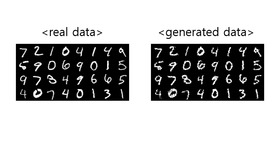
Figure 5. Results of training the RBM. Original data fed into the visible layer and data obtained through sampling in the visible layer.

References

• Introduction to Restricted Boltzmann Machine, Edwin Chen
• Restricted Boltzmann Machine, DeepLearning 0.1 Documentation
• What is the difference between autoencoders and a restricted Boltzmann machine?
• Ali Ghodsi, Lec [7], Deep Learning , Restricted Boltzmann Machines (RBMs)