Prerequisites

To understand this post well, it is recommended to have knowledge about the following topics:

• Basic operations of vectors
• Eigenvalues and eigenvectors
• Linear algebra and Fourier transform
• Eigenvalue decomposition (EVD)
• Circulant matrices and convolution

Eigenvalues and eigenvectors of permutation matrices

The eigenvalues and eigenvectors of circulant matrices are closely related to those of permutation matrices.

Therefore, let’s first calculate the eigenvalues and eigenvectors of a permutation matrix.

The permutation matrix we use is a matrix that performs a cyclic permutation as seen in the Circulant matrices and convolution article, as shown below:

\[P = \begin{bmatrix} 0 & 0 & \cdots & 0 & 1 \\ 1 & 0 &\cdots & 0 & 0 \\ 0 & \ddots &\ddots & \vdots & \vdots \\ \vdots & \ddots & \ddots & 0 & 0 \\ 0 & \cdots & 0 & 1 & 0\end{bmatrix}\]

Calculating the eigenvalues and eigenvectors of a general $n\times n$ matrix $P$ can be difficult, so let’s calculate the eigenvalues and eigenvectors of a $4\times 4$ permutation matrix $P_4$.

First, to calculate the eigenvalues of $P_4$, we can write the characteristic equation as follows:

\[det(P_4-\lambda I) = 0\] \[\Rightarrow det\left(\begin{bmatrix}0 & 0 & 0 & 1 \\ 1 & 0 & 0 & 0 \\ 0 & 1 & 0 & 0 \\ 0 & 0 & 1 & 0\end{bmatrix}-\lambda I\right)=0\] \[\Rightarrow det\left(\begin{bmatrix}-\lambda & 0 & 0 & 1 \\ 1 & -\lambda & 0 & 0 \\ 0 & 1 & -\lambda & 0 \\ 0 & 0 & 1 & -\lambda\end{bmatrix}\right)=0\]

Determinants of matrices larger than $3\times 3$ can be calculated using the adjugate matrix.

That is,

\[\Rightarrow 1\times (-\lambda)\times det\left(\begin{bmatrix}-\lambda & 0 & 0 \\ 0 & -\lambda & 0 \\ 0 & 0 & -\lambda \end{bmatrix}\right)-1\times(1)\times det\left(\begin{bmatrix} 1 & -\lambda & 0 \\ 0 & 1 & -\lambda \\ 0 & 0 & 1 \end{bmatrix}\right) = 0\] \[\Rightarrow \lambda^4 - 1 = 0\]

Therefore, the eigenvalues of $P_4$ are $\lambda = 1, -1, i, -i$.

Let’s use this to calculate the eigenvectors.

1) When $\lambda = 1$,

We need to satisfy $P_4v=\lambda v$, so

\[(P_4-\lambda I)v = (P_4-I)v = 0\]

and if we assume $v = [v_1, v_2, v_3, v_4]^T$,

\[\begin{bmatrix} -1 & 0 & 0 & 1 \\ 1 & -1 & 0 & 0 \\ 0 & 1 & -1& 0 \\ 0 & 0 & 1 & -1\end{bmatrix}\begin{bmatrix}v_1\\v_2\\v_3\\v_4\end{bmatrix} = 0\]

should hold, so the eigenvector $v$ satisfying the relationship $v_1=v_4$, $v_1 = v_2$, $v_2=v_3$, $v_3 = v_4$ is

\[v=\begin{bmatrix}1\\1\\1\\1\end{bmatrix}\]

2) When $\lambda = -1$,

By following a similar method to the case when $\lambda = 1$,

\[\begin{bmatrix} 1 & 0 & 0 & 1 \\ 1 & 1 & 0 & 0 \\ 0 & 1 & 1& 0 \\ 0 & 0 & 1 & 1\end{bmatrix}\begin{bmatrix}v_1\\v_2\\v_3\\v_4\end{bmatrix} = 0\]

should hold, and the eigenvector satisfying the relationship $v_1=-v_4$, $v_1 = -v_2$, $v_2=-v_3$, $v_3 = -v_4$ is

\[v=\begin{bmatrix}1\\-1\\1\\-1\end{bmatrix}\]

3) When $\lambda = i$,

Using a similar method as the above two cases, we can see that the eigenvector is

\[v = \begin{bmatrix}1 \\ i \\ i^2 \\ i^3 \end{bmatrix}\]

4) In the case of $\lambda=-i$, the eigenvector can be obtained through a method similar to the two methods above:

\[v = \begin{bmatrix}1 \\ (-i) \\ (-i)^2 \\ (-i)^3 \end{bmatrix}\]

Generally, the eigenvalues of a permutation matrix of size $n\times n$ can be expressed as $\lambda^n-1=0$, where $\lambda$ satisfies this equation ¹:

\[\lambda_k = \exp\left(-j\frac{2\pi}{n}k\right)\text{ for } k = 0, 1, \cdots ,n-1\]

The corresponding eigenvectors for each eigenvalue are as follows:

\[v_k = \begin{bmatrix}(\lambda_k)^0 \\ (\lambda_k)^1\\ \vdots \\ (\lambda_k)^{n-1}\end{bmatrix}\text{ for } k = 0, 1, \cdots ,n-1\]

Eigenvectors of cyclic matrices

\[C= \begin{bmatrix} x_0 & x_{n-1} & \cdots & x_2 & x_1 \\ x_1 & x_1 &\cdots & x_3 & x_2 \\ x_2 & \ddots &\ddots & \vdots & \vdots \\ \vdots & \ddots & \ddots & x_0 & x_{n-1} \\ x_{n-1} & \cdots & x_2 & x_1 & x_0\end{bmatrix} = \left(\sum_{i=0}^{n-1}x_i P^{i}\right)\]

The eigenvectors of a cyclic matrix are the same as those of a permutation matrix.

The eigenvalue $\lambda$ and eigenvector $v$ of $P$ satisfy the following equation:

\[Pv=\lambda v\]

If we denote the eigenvector of the cyclic matrix $C$ as $v$, it should satisfy the following equation with the eigenvalue $\xi$ of the cyclic matrix:

\[Cv=\xi v\]

Based on the relationship between cyclic matrices and permutation matrices, the above equation can be expressed as:

\[Cv = x_0 I v + x_1 P^1 v + \cdots + x_{n-1}P^{n-1}v\] \[=x_0 \lambda^0 v + x_1 \lambda^1 v + \cdots + x_{n-1}\lambda^{n-1}v\] \[=\left(\sum_{i=0}^{n-1}x_i\lambda^i\right)v = \xi v\]

In other words, the eigenvectors of cyclic matrices and permutation matrices are the same.

Understanding Fourier matrix based on the transformation of basis

Let’s think about the ‘basis’ that represents vectors.

In the previous article about basic vector operations, we briefly mentioned the characteristics of vectors. The first two were that ‘vectors are like arrows’ and ‘vectors are ordered sequences of numbers.’

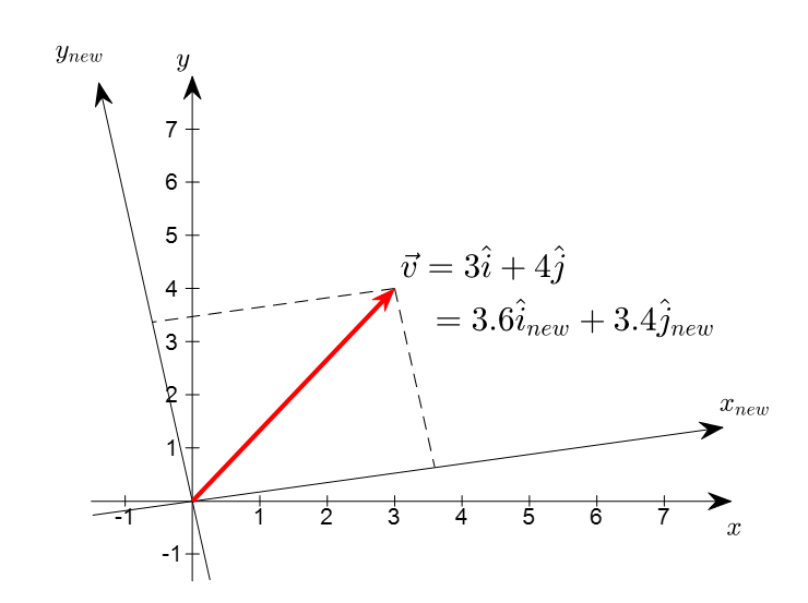
Figure 1. Geometric characteristics of vectors that are invariant to changes in the coordinate system

From Figure 1, we can see that we can represent a single vector using a completely different coordinate system.

Also, depending on the coordinate system used, the sequence of numbers used to represent the vector can be either concise or complex.

Therefore, we can easily handle data (i.e., vectors) by selecting an appropriate coordinate system.

The basic unit of the coordinate system mentioned here is called the ‘basis.’ In other words, if we choose the appropriate basis for our purpose, we can represent the same vector (i.e., given data) more easily or usefully.

The basis that we have commonly used so far can be called the standard basis. For example, for the vector $\vec{x}$ below,

\[\vec{x} = \begin{bmatrix}x_0\\x_1\\ \vdots \\ x_{n-1}\end{bmatrix}\]

using the standard basis means representing the vector $\vec{x}$ using basis vectors filled with 1 and 0 as shown below.

\[\begin{bmatrix}x_0\\x_1\\ \vdots \\ x_{n-1}\end{bmatrix} = x_0 \begin{bmatrix}1\\0\\ \vdots \\ 0\end{bmatrix} + x_1 \begin{bmatrix}0\\1\\ \vdots \\ 0\end{bmatrix} + \cdots + x_{n-1} \begin{bmatrix}0\\0\\ \vdots \\ 1\end{bmatrix}\]

Meanwhile, according to what we have seen so far, any vector can be thought of as the product of a circulant matrix $C$ and a $\delta$ vector, which means that any signal can be seen as the result obtained by transforming the $\delta$ vector.

\[\vec{x} = C\delta=\left(\sum_{i=0}^{n-1}x_i P^{i}\right)\delta\]

(Under construction…)