※ The content of this post is largely borrowed from Thomas Judson’s The ordinary differential equations project

In the previous post on separation of variables, we solved separable differential equations, the simplest form of first-order linear differential equations.

This time, we want to learn about the solution to a more general form of first-order linear differential equations that cannot be solved by separation of variables.

The form of the differential equation we want to solve is as follows:

\[\frac{dx}{dt}+p(t)x=q(t) % Equation (1)\]

The difference between Equation (1) and the equation we saw in separation of variables is that the $p(t)$ in the middle is no longer a constant.

If $p(t)$ is not a function of $t$, we can solve the problem by separation of variables.

Meaning of ‘linear’

When we study differential equations, we often hear about linear differential equations.

Later, we will often hear about the fact that differentiation is a ‘linear operator.’

We will cover this in more detail when we introduce the Sturm-Liouville problem later, but for now, let’s just understand the meaning of ‘linear.’

---

First, we need to understand the concept of an operator.

When we study differential equations, the ‘operator’ we think of refers to a function that transforms a given function into another function.

We can think of it as an ‘agent’ that transforms a function into another function.

In other words, we can think of Equation (1) as follows. Let’s consider an arbitrary operator $O(\cdot)$. When this operator acts on a function $x(t)$, it produces the following output:

\[x(t)\rightarrow O(\cdot) \rightarrow \frac{dx}{dt}+p(t)x % Equation (2)\]

If this operator is a ‘linear’ operator, it must satisfy the following properties:

For any constant $c$,

\[O(c\cdot x(t))=c\cdot O(x(t)) % Equation (3)\]

Also, for two independent functions $x_1(t)$ and $x_2(t)$,

\[O(x_1(t) + x_2(t)) = O(x_1(t)) + O(x_2(t)) % Equation (4)\]

Therefore, if the operator $O(\cdot)$ is a linear operator, the following result can be derived¹.

For arbitrary constants $c_1$ and $c_2$,

\[O(c_1 x_1(t) + c_2 x_2(t)) = c_1 O(x_1(t)) + c_2 O(x_2(t)) % equation (5)\]

Again, the meaning of a linear differential equation is that the operator, such as in equation (2), is a linear operator. That is, for independent functions $x_1(t)$ and $x_2(t)$,

\[\frac{d}{dt}\left(c_1x_1(t) + c_2x_2(t)\right)+p(t)\left(c_1x_1(t) + c_2x_2(t)\right) % equation (6)\] \[=c_1\frac{dx_1}{dt}+c_1p(t)x_1(t) + c_2\frac{dx_2}{dt}+c_2p(t)x_2(t) % equation (7)\]

This is why the name “linear differential equation” is given.

Example of a nonlinear differential equation

Let’s take an example to check when the differential operator is nonlinear. The following differential equation is a nonlinear differential equation.

\[\frac{dx}{dt}+x^2 = 0\]

Because the following two equations do not match.

\[O(c_1 x_1 + c_2 x_2 ) = c_1 \frac{dx_1}{dt}+c_1^2 x_1^2 + c_2 \frac{dx_2}{dt}+c_2^2x_2^2+2c_1x_1c_2x_2\] \[\neq c_1O(x_1)+c_2O(x_2) = c_1 \frac{dx_1}{dt}+c_1x_1^2+c_2\frac{dx_2}{dt}+c_2 x_2^2\]

Solution of first-order linear differential equations

To solve a differential equation of the form shown in equation (1), we need to use the chain rule of differentiation.

Let us consider a function $\mu(t)$ that satisfies the relationship $\mu’(t) = p(t)$ or $\int p(t) dt = \mu(t)$ with respect to the $p(t)$ in the middle of equation (1).

Then, we can write the derivative of $e^{\mu(t)}x$ with respect to $t$ as follows:

\[\frac{d}{dt}\left(e^{\mu(t)}x(t)\right)=e^{\mu(t)}\mu'(t)x(t) + e^{\mu(t)}x'(t) % equation (11)\] \[=e^{\mu(t)}\left\lbrace \mu'(t)x(t)+x'(t)\right\rbrace % equation (12)\] \[=e^{\mu(t)}\left\lbrace p(t)x(t) + x'(t)\right\rbrace % equation (13)\]

The expression inside the curly braces of equation (13) is ultimately equal to the left-hand side of equation (1). Therefore,

\[\text{equation (11)}\Rightarrow \frac{d}{dt}\left(e^{\mu(t)}x(t)\right) = e^{\mu(t)}q(t)\] \[\therefore e^{\mu(t)}x(t)=\int e^{\mu(t)}q(t)dt + C\]

That is,

\[x(t) = \frac{1}{e^{\mu(t)}}\left(\int e^{\mu(t)}q(t)dt + C\right)\]

We can see that an important point here is that the process of multiplying $e^{\mu(t)}$ to $x$ is where this solution starts. $e^{\mu(t)}$ is called the integrating factor.

Sample Problem

Since it is important to understand how the solution of differential equations works, it is important to solve many problems.

Saltwater Tank Filling Problem

Let’s solve the saltwater tank filling problem by upgrading the problem we saw in the Separable Differential Equations posting.

Unlike the previous Separable Differential Equations posting, this time we will modify the problem so that the water level can continue to rise.

Suppose we add saltwater to a water tank to increase the salinity of the water in the tank.

For example, let’s say there is a total volume of 1000 liters in the water tank, and 500 liters of fresh water is already in it, and we start adding 0.5kg/L concentrated saltwater continuously.

At this point, let’s say that 10L of 0.5kg/L concentrated saltwater is continuously added per minute.

Assume that the saltwater in the water tank is uniformly mixed by constantly stirring the water in the water tank.

However, let’s say that water is leaking from the bottom of the water tank. Let’s assume that the rate of water leakage is 9L per minute.

In this case, how will the concentration of saltwater change over time?

---

This problem requires the use of differential equations and a first-order linear differential equation must be used.

Let’s call the amount of salt inside the water tank $x(t)$. Then, the rate of change of the amount of salt inside the water tank with respect to time will be $dx/dt$.

Also, the rate of change of salt per unit time is the difference between the rate of salt coming in and the rate of salt going out, so we can write it as follows:

\[\frac{dx}{dt}=\text{rate in } - \text{rate out} % Equation (17)\]

The incoming saltwater is 10L, and 5kg of it is salt, so 5kg of salt comes in per minute. That is,

\[\text{rate in}=5\]

Meanwhile, the volume $V(t)$ of saltwater in the water tank, which was initially 500 liters, increases by 1 liter per minute because 10 liters of water flow in and 9 liters of water flow out. Therefore, $V(t)$ can be expressed as $V(t) = 500 + t$.

Therefore, the amount of salt leaving the tank will be proportional to the current amount of salt $x$ in the tank and inversely proportional to the current volume of water in the tank $V(t)$. In other words,

\[\text{rate out}=\frac{9}{500+t}x\]

Thus, we can set up a differential equation as follows:

\[\frac{dx}{dt}=5-\frac{9}{500+t}x \qquad \text{(Equation 20)}\]

Rearranging Equation 20, we get:

\[\Rightarrow \frac{dx}{dt}+\frac{9}{500+t}x=5 \qquad \text{(Equation 21)}\]

Multiplying both sides of Equation 21 by the integrating factor $e^{\mu(t)}$, we get:

\[e^{\mu(t)}=\exp\left(\int \frac{9}{500+t}dt\right)=e^{9\ln(500+t)}=(500+t)^9\]

Thus, multiplying both sides of Equation 21 by the integrating factor $e^{\mu(t)}$, we get:

\[\Rightarrow (500+t)^9\frac{dx}{dt}+9(500+t)^8x=5(500+t)^9\] \[\Rightarrow \frac{d}{dt}\left[(500+t)^9x\right]=5(500+t)^9\]

Integrating both sides yields:

\[(500+t)^9x=\frac{5}{10}(500+t)^{10}+C\] \[\therefore x(t) = \frac{1}{2}(500+t)+\frac{C}{(500+t)^9}\]

The initial water in the tank had no salt in it, so:

\[x(0) = \frac{1}{2}(500+0)+\frac{C}{(500+0)^9}=250+\frac{C}{500^9}=0\]

Thus,

\[C = -250 * 500^9=-\frac{1}{2}\times 500^{10}\]

as a result.

The graph of the amount of salt up to the time it takes for a water tank to be filled up with water after 500 minutes will look like this.

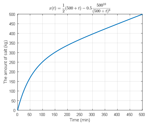
Figure 1. Changes in the amount of salt in the water tank when gradually filling it with salt water in a leaking water tank.

Existence and uniqueness of solutions

When solving differential equations, it is helpful to be aware that, by guaranteeing the existence and uniqueness of solutions, we can obtain solutions regardless of the method used to find them.

(In other words, this can be an answer to the question of why we need to know the solution acquisition methods that others have thought of.)

In most cases, the existence and uniqueness of solutions for first-order linear differential equations can be guaranteed. Specifically, under the following conditions:

\[y'+p(t)y = g(t)\]

For the first-order linear differential equation with the initial condition of $y(t_0)=y_0$, and $p(t)$ and $g(t)$ being continuous on the open interval $I=(\alpha, \beta)$, there exists a unique function $y=\phi(t)$ that satisfies the initial condition in this interval.

This is because, considering that $p(t)$ and $g(t)$ are continuous on the interval $I$, we can define the integral expression in Equation (11), and the constant of integration $C$ can be uniquely determined according to the initial condition.