Deep Neural Network Transparency

Neural networks have traditionally been considered as “Blackbox” models. In my opinion, there are two main reasons for this. First, neural networks are inherently non-linear regression models, making it difficult to directly understand how inputs affect outputs due to the lack of linearity in the relationship between them. Moreover, with recent advancements in deep learning, neural networks are now capable of selecting relevant features for classification/regression from complex high-dimensional data on their own, eliminating the need for developers to manually engineer features.

As the performance of neural networks continues to improve and attempts to apply them in real-world fields increase, it is crucial to understand how the algorithms work in order to ensure their reliability when deployed. Research aimed at understanding how neural networks operate can be broadly categorized into two types. The first type involves interpreting the model itself, while the second type involves understanding the reasoning behind the decisions made by the model.

Figure 0. Classification of various methods for understanding the operation of neural networks
Source: ICASSP2017 Tutorials on Methods for Interpreting and Understanding Deep Neural Networks

In this article, we will explore Layer-wise Relevance Propagation (LRP), which belongs to the second type of research that aims to understand the reasoning behind the decisions made by neural networks, and specifically utilizes decomposition as a method.

Goal of LRP

LRP is a method that helps understand the output of a neural network through explanation by decomposition.

To be more specific, the goal of LRP is to calculate relevance scores for each dimension of the $d$-dimensional input $x = (x_1, x_2, \cdots, x_i, \cdots, x_d)$ with respect to the output obtained by the trained neural network model, denoted as $f(x)$.

At this point, the relevance score for each dimension i has the following characteristics:

\[f(x) = \sum_{i=1}^{d}R_i\]

To help with understanding, let’s think of the input sample x as an image. If we input a photo of a rooster into a well-trained neural network and obtain the output ‘rooster’, the relevance scores ($R_i$) for each pixel of the input sample that contribute to the output f(x)¹ are calculated.

As shown in Figure 1, the heatmap labeled as “heatmap” displays the relevance (relevance score) of each pixel in terms of color, and we can see that the output classified the input as ‘rooster’ based on the beak and head of the rooster.

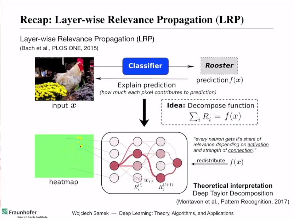
Figure 1. Summary of how LRP works and its results
Source: Explaining Decisions of Neural Networks by LRP. Alexander Binder @ Deep Learning: Theory, Algorithms, and Applications. Berlin, June 2017

The intuition behind it

As the name suggests, LRP (Layer-wise Relevance Propagation) is a method that redistributes relevance scores from the output layer to the input layer in a top-down manner.

The basic assumptions and operation of LRP are as follows:

• Each neuron has a certain amount of relevance (certain relevance).
• Relevance is redistributed from the output layer to the input layer in a top-down manner.
• The relevance is preserved during (re)distribution.

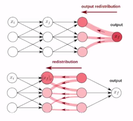
Figure 2. Distribution process of relevance scores
Source: Explaining Decisions of Neural Networks by LRP. Alexander Binder @ Deep Learning: Theory, Algorithms, and Applications. Berlin, June 2017

If we further explain the statement that the relevance is preserved during redistribution, for example, let’s say we classified a specific input image as ‘rooster’ with an output value (which can be interpreted as probability) of $f(x) = 0.9$ as shown in Figure 1. Then, the neurons in each layer should all have some relevance to the output value of 0.9, and after distributing the relevance scores, the sum of the relevance scores in each layer should be 0.9.

Explanation for neural network?

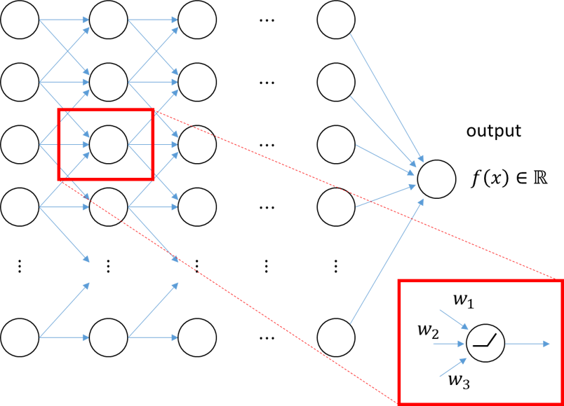
Figure 3. You can decompose the prediction or output value ($f(x)$) of a deep neural network by examining the output values of each neuron on the network.

Now, the practical problem we face is this: How can we mathematically decompose the prediction or output value ($f(x)$) of a deep neural network and define ‘relevance’?

The solution to this problem is to think about it neuron by neuron, following the “basic assumptions and operating principles” explained above, and particularly, to define relevance mathematically using the relationship between the output and input of each neuron.

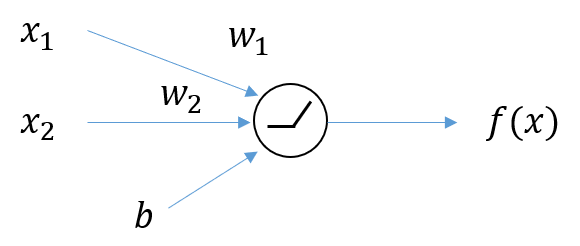
Figure 4. A neuron with 2-dimensional input and 1-dimensional output.

Let’s consider a basic neuron with 2 inputs (i.e., 2 weights and 1 bias) as shown in Figure 4.

Mathematically, the relevance score can be viewed as the degree of change in the output with respect to the change in the input.

In other words, the relevance of each input $x_1, x_2$ to the output $f(x)$ in Figure 4 can be expressed as follows:

\[\frac{\partial f}{\partial x_1}, \frac{\partial f}{\partial x_2}\]

Therefore, if we can derive an appropriate equation that explains the relationship between $f(x)$ and $\frac{\partial f}{\partial x_1}, \frac{\partial f}{\partial x_2}$, we can think of decomposing the output into relevance scores.

LRP introduces the Taylor Series for this purpose.

Taylor Series

For any smooth function $f(x)$ and a real number $a$, the Taylor Series of $f(x)$ is given as follows.

\[f(x) = \sum_{n=0}^{\infty}\frac{f^{(n)}(a)}{n!}(x-a)^n\] \[=f(a) + \frac{f'(a)}{1!}(x-a) + \frac{f''(a)}{2!}(x-a)^2 + \frac{f'''(a)}{3!}(x-a)^3 + \cdots\]

Using the error term “$\epsilon$,” the first-order Taylor series can be written as follows.

\[f(x) = f(a) + \frac{d}{dx}f(x)\big|_{x=a}(x-a) + \epsilon\]

For multivariate functions, the Taylor series can be expressed as follows.

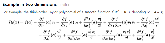
Figure 5. Taylor series for multivariate functions. Source: Wikipedia

In other words, for d-dimensional inputs, the first-order Taylor series can be written as follows.

\[f(\pmb{x}) = f(\pmb{a}) + \sum_{p = 1}^{d}\frac{\partial \pmb{f}}{\partial x_p}\big|_{\pmb{x}=\pmb{a}}(\pmb{x} - \pmb{a}) + \epsilon\]

The second term on the right-hand side of the equation represents how much $f(x)$ changes when $x_p$ changes.

‘Appropriate’ Modification of the Taylor Series Formula

Equation (6) has two unnecessary terms, namely $f(a)$ and $\epsilon$, that can be mathematically set to zero using the properties of the Taylor series. By approximating the function from the point $a$ where $f(a) = 0$, and utilizing the properties of the ReLU activation function, $\epsilon$ can also be set to zero.

If we can do that, the output $f(x)$ can be decomposed into relevance scores as follows.

\[f(x) = f(a) + \sum_{i=1}^{d}\frac{\partial f}{\partial x_i}\big|_{x_i = a_i}(x_i-a_i) + \epsilon\] \[= \sum_{i=1}^{d}\frac{\partial f}{\partial x_i}\big|_{x_i = a_i}(x_i-a_i)\] \[= \sum_{i=1}^{d}R_i\]

Let’s confirm that epsilon = 0 through the characteristics of ReLU.

The operation of a neuron with ReLU activation function can be mathematically described as follows, with two inputs and one output, as shown in Figure 4:

\[f(x) = \max\left(0, \sum_{i=1}^{2}w_i x_i + b\right)\] \[= \begin{cases}0 & \text{case i) when $\sum_{i=1}^{2}w_ix_i + b \leq 0$} \\\sum_{i=1}^{2}w_ix_i + b & \text{case ii) when $\sum_{i=1}^{2}w_ix_i + b > 0$}\end{cases}\]

As seen in equation (11), we can see that we no longer need to consider case i), and we can continue to expand the expression for case ii).

On the other hand, the function $f(x)$ in equation (10) can also be expressed as a Taylor series, as shown in equation (7). Therefore,

\[f(x) = \sum_{i=1}^{2}w_ix_i + b = f(a) + \sum_{i=1}^{d}\frac{\partial f}{\partial x_i}\big|_{x_i=a_i}(x_i-a_i) + \epsilon\]

Looking closely at equation (12), we can express $f(x)$ as follows:

\[f(x) = w_1x_1+w_2x_2+b\]

Therefore, the partial derivatives of $f(x)$ with respect to $x_i$ are as follows:

\[\frac{\partial f(x)}{\partial x_1}= w_1, \frac{\partial f(x)}{\partial x_2} = w_2\]

Furthermore, all second or higher order partial derivatives are equal to 0:

\[\frac{\partial ^2 f(x)}{\partial x_1 ^2} = 0, \space \frac{\partial^2 f(x)}{\partial x_1 \partial x_2} = 0, \space \cdots\]

Hence, from the Taylor series representation in equation (12), we can conclude that $\epsilon=0$.

Therefore, we can rewrite equation (12) as follows:

\[f(x) = \sum_{i=1}^{2}w_ix_i+b = f(a) + \sum_{i=1}^{2}w_i(x_i-a_i)\]

Finding the appropriate $a$

When approximating a function using Taylor series, if we can add an infinite number of terms regardless of the position of the starting point $x=a$, we can accurately approximate the function.

However, in LRP, as seen in equation (8), the constraint $f(a)=0$ exists. Therefore, we need to find an $a$ that satisfies this constraint, and there may still be infinitely many $a$ that can satisfy this constraint.

The method we will introduce this time is the $w^2$-rule, introduced in the reference (Explaining NonLinear Classification ~).

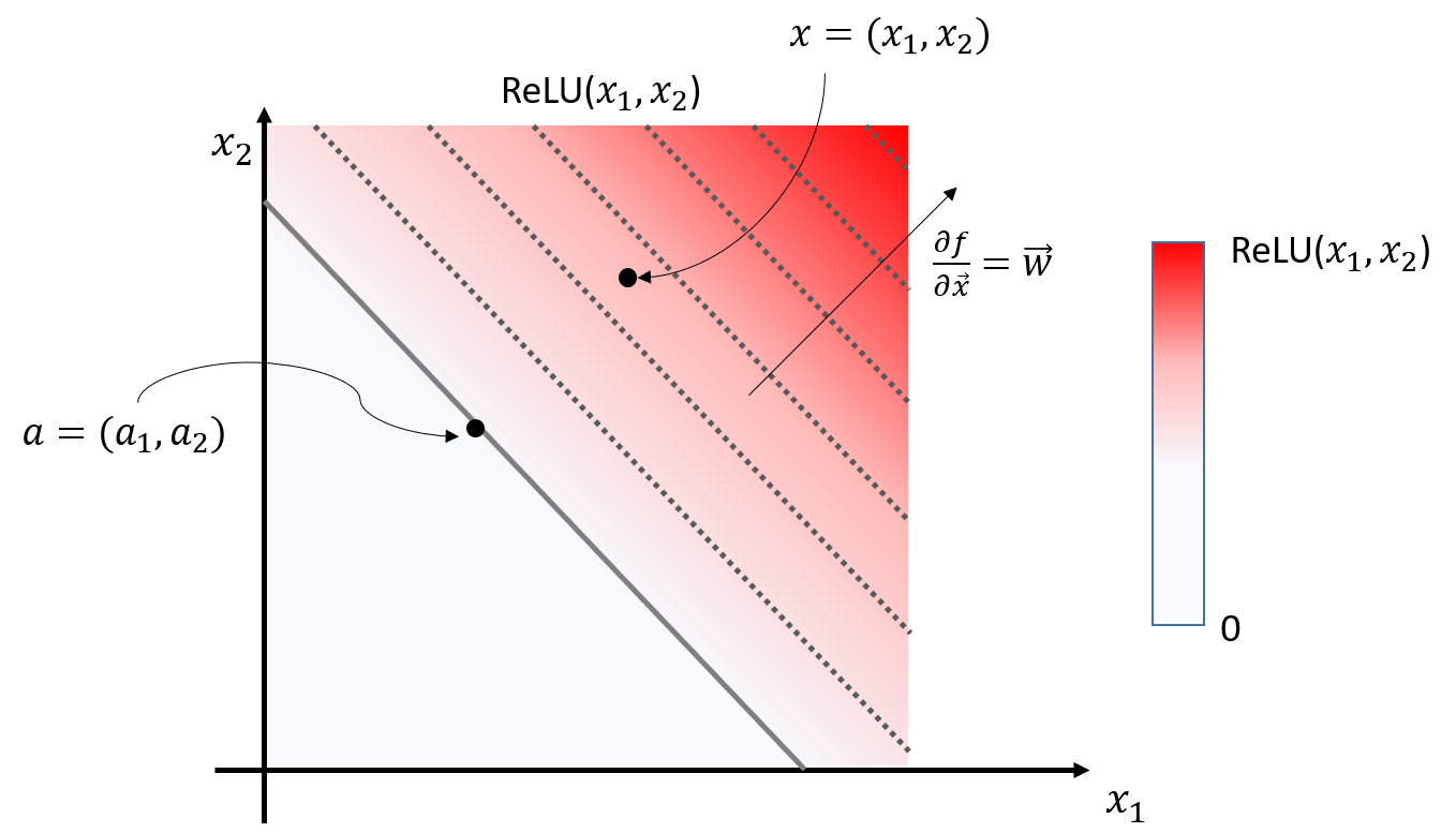
Figure 6. Diagram depicting the input-output relationship of a neuron with two inputs and one output value after passing through ReLU

Figure 6 represents the input-output relationship of a neuron with two inputs and one output value, similar to the neuron depicted in Figure 4. The inputs $x_1, x_2$ are known values that we input, and the output value $f(x_1, x_2) = ReLU(x_1, x_2)$ is determined by the neural network model. The output value is represented by color, where values closer to white are closer to 0, and values closer to red are larger. The solid lines represent points where all values are 0, and the dotted lines represent contour lines with the same value.

As seen in Figure 6, the appropriate $a$ according to the $w^2$-rule is the point where the output value is 0 (i.e., $f(a) = 0$) and closest to the input $x = (x_1, x_2)$.

When following the $w^2$-rule, we can go through the following process to calculate $a$.

Considering the meaning of the arrows in Figure 6, $\vec{a}$ and $\vec{x}$ have the following relationship:

\[\vec{a} - \vec{x} = t\vec{w}\]

In other words, the vector obtained by subtracting $\vec{x}$ from $\vec{a}$ should be a scalar multiple of $\vec{w}$.

If we slightly modify this equation,

\[\vec{a} = \vec{x} + t\vec{w}\]

Now, according to our constraint ($f(a) = 0$),

\[f(\vec{a}) = \sum_{i=1}w_ia_i+b = 0\]

Substituting equation (18) into equation (19),

\[f(\vec{a}) = \sum_{i=1} w_i(x_i+tw_i) + b = 0\] \[= \sum_{i=1}w_ix_i + t\sum_{i}w_i^2 + b = 0\]

\(\therefore t = - \frac{\sum_i w_ix_i + b}{\sum_i w_i^2}\) If you substitute equation (22) into equation (18), you get:

\[a_i = x_i - \left( \frac{\sum_iw_ix_i + b}{\sum_iw_i^2} \right)w_i\]

Using equation (23), you can express $f(x)$ as follows:

\[f(x) = 0 + \sum_i w_i\left(\frac{\sum_iw_ix_i + b}{\sum_i w_i^2}\right)w_i + 0\] \[=\sum_i\left(\frac{\sum_iw_ix_i + b}{\sum_i w_i^2}\right)w_i^2 = \sum_iR_i\]

Note that besides the $w^2$-rule, there are various other rules such as the $z$-rule, $z^+$-rule, etc. It is recommended to refer to the literature (Explaining NonLinear ~) for more information.

Summary of Relevance Propagation Rule

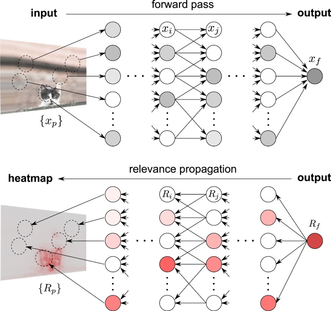
Figure 7. Visualization of Forward Pass and Relevance Propagation in a single image.

Based on the summary of the content so far, it can be concluded that the output $f(x)$ of a single neuron can be decomposed as follows:

\[f(x) = \sum_i R_i\]

If you want to apply the insights obtained for a single neuron to the entire neural network as shown in Figure 7, you can follow the following process:

Let’s assume that the final output of the neural network for a specific input ${x_p}$ is denoted as $x_f$ (forward pass) as shown in the top part of Figure 7.

Then, let’s set the relevance score $R_f$ of the output neuron to be equal to $x_f$, and propagate it backwards to the previous layers.

In other words, by thinking of $R_f = \sum_i R_i$ similar to the equation $f(x) = \sum_i R_i$, you can calculate the relevance scores of all neurons in the neural network by propagating backwards through the layers.

Python Code for Reference

# -------------------------
# Feed-forward network
# -------------------------
class Network:
    def __init__(self,layers):
        self.layers = layers
    
    def forward(self,Z):
        for l in self.layers: Z = l.forward(Z)
        return Z
    
    def gradprop(self,DZ):
        for l in self.layers[::-1]: DZ = l.gradprop(DZ)
        return DZ
    
    def relprop(self, R):
        for I in self.layers[::-1]: R = I.relprop(R)
        return R

# -------------------------
# ReLU activation layer
# -------------------------
class ReLU:
    def forward(self,X):
        self.Z = X>0
        return X*self.Z
    
    def gradprop(self,DY):
        return DY*self.Z
    
    def relprop(self, R): 
        return R
    
# -------------------------
# Fully-connected layer
# -------------------------
class Linear:

  def __init__(self, weight, bias):
    self.W = weight
    self.B = bias

  def forward(self,X):
    self.X = X
    return np.dot(self.X,self.W)+self.B

  def gradprop(self,DY):
    self.DY = DY # You can put target for DY. Desired Y
    return np.dot(self.DY,self.W.T)


class NextLinear(Linear): # implementing Z+ rule
    def relprop(self,R):
        V = np.maximum(0,self.W) # V means W_ij^+
        Z = np.dot(self.X,V)+1e-9; S = R/Z
        C = np.dot(S,V.T);         R = self.X*C
        return R
    
class FirstLinear(Linear): # implementing Zbeta rule
    def relprop(self,R):
        W,V,U = self.W,np.maximum(0,self.W),np.minimum(0,self.W)
#        X,L,H = self.X,self.X*0+utils.lowest,self.X*0+utils.highest
        X,L,H = self.X,self.X*0+(-1),self.X*0+(1.0)


        Z = np.dot(X,W)-np.dot(L,V)-np.dot(H,U)+1e-9; S = R/Z
        R = X*np.dot(S,W.T)-L*np.dot(S,V.T)-H*np.dot(S,U.T)
        return R

# Creating a Neural Network Structure
nn = Network([
    FirstLinear(final_W1, final_b1),ReLU(),
    NextLinear(final_W2, final_b2),ReLU(),
    NextLinear(final_W3, final_b3),ReLU(),
    NextLinear(final_W4, final_b4),ReLU(),
    NextLinear(final_Wh, final_bh),ReLU(),
])

rand_num = np.random.permutation(n_total)

X = total_x[rand_num,:] # Input
T = total_y[rand_num,:] # Target
Y = nn.forward(X) # Output
S = nn.gradprop(T)**2
Y = nn.forward(X)

D = nn.relprop(Y*T)

Reference

• Explaining NonLinear Classification Decisions with Deep Taylor Decomposition, Montavon et al., 2015
• Explaining Decisions of Neural Networks by LRP. Alexander Binder @ Deep Learning: Theory, Algorithms, and Applications. Berlin, June 2017
• ICASSP2017 Tutorials on Methods for Interpreting and Understanding Deep Neural Networks