Relationship between the location of poles and basis function $\exp(\sigma t)$
Source: MIT Mathlets, https://mathlets.org/mathlets/poles-and-vibrations/

Relationship between pole diagram and frequency response
Source: MIT Mathlets, https://mathlets.org/mathlets/amplitude-response-pole-diagram/

Prerequisites

To better understand this blog post, it is recommended that you have knowledge of the following topics:

• Signal Space
• Continuous Time Fourier Series
• Comtinuous Time Fourier Transform

In the following content, $\delta(t)$ represents the Dirac delta function.

\[\delta(t) =\begin{cases} \infty, && t = 0 \\ 0 && \text{otherwise}\end{cases}, \quad \int_{-\infty}^{\infty}\delta(t)dt = 1\]

Also, $u(t-t_0)$ represents the unit step function.

\[u(t-t_0)=\begin{cases} 1 && t \geq t_0 \\ 0 && \text{otherwise}\end{cases}\]

Limitations of Fourier Transform

Studying Fourier series and Fourier transform, we learned how to analyze the frequency characteristics of continuous-time signals. In addition, the Fourier analysis methods can be applied very effectively to Linear Time-Invariant (LTI) systems, allowing us to understand the frequency response characteristics of LTI systems by applying Fourier transform to their impulse response.

However, there are conditions that must be met to use Fourier series or transform. It is called the Dirichlet condition, which essentially requires that the signal to be transformed must be absolutely integrable. In other words, if the signal to be transformed is a signal, it must be a signal that does not diverge, and if it is an impulse response, it means that only the impulse response of a stable system can be analyzed using Fourier analysis.

For example, signals such as $x(t) = e^{at}\cos(b t)u(t), \text{ for }a\gt 0$ or impulse responses of systems with such characteristics do not have Fourier transforms, and therefore, frequency analysis through Fourier analysis cannot be performed as the magnitude of the signal diverges to infinity as time progresses.

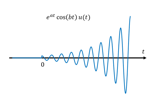
Figure 1. Diverging cosine wave over time

However, even for unstable systems, frequency analysis can be very useful. For example, it allows us to determine how quickly a signal or impulse response diverges, and at what frequency it oscillates.

Pierre-Simon Laplace (1749-1827) came up with a transformation that could generalize the Fourier transform and overcome this limitation¹.

The idea behind Laplace transform

The idea is very simple. Assume an arbitrary real number $\sigma$ and multiply the signal by an appropriate $\exp(-\sigma t)$ that cancels out the oscillating term, and then take the Fourier transform of the resulting signal.

Figure 2. Core of the Laplace transform: Multiplying the signal by a decaying exponential term to prevent divergence and enable Fourier transformation

For example, consider $x(t) = e^{2t}\cos(3t)u(t)$, where $u(t)$ is the unit step function. This signal still diverges over time, but if we multiply it by $e^{-2t}$, we get $x(t)e^{-2t}=\cos(3t)u(t)$, which has a Fourier transform.

However, in practice, knowing the appropriate value of $\sigma$ is virtually impossible when we have an arbitrary signal $x(t)$. Therefore, in Laplace transform, we multiply the signal by $\exp(-\sigma t)$ for all possible $\sigma\in\mathbb{R}$ and then take the Fourier transform of the resulting signals. This allows us to gather all the transformed signals for different $\sigma$ on a single plane, as shown in the following figure.

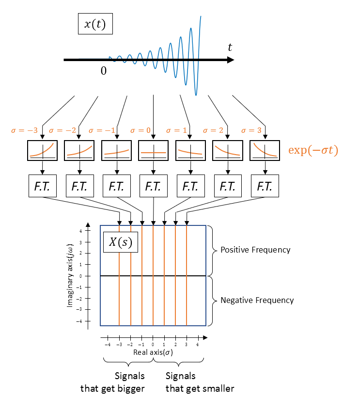
Figure 3. Laplace transform is the collection of Fourier transforms of the input signal multiplied by exponential functions that decay or diverge.

Therefore, the Laplace transform is a slight modification of the Fourier transform, which can be written as follows.

Let’s assume the original Fourier transform is as follows.

\[X(\omega) = \int_{-\infty}^{\infty}x(t)\exp(-j\omega t)dt\]

If we perform the Fourier transform with $x(t)\exp(-\sigma t)$ instead of $x(t)$, then we have:

\[X(\sigma, \omega)=\int_{-\infty}^{\infty}x(t)\exp(-\sigma t)\exp(-j\omega t)dt\] \[= \int_{-\infty}^{\infty}x(t)\exp(-(\sigma+j\omega)t)dt\]

Let’s denote $\sigma+j\omega$ as a new variable $s=\sigma+j\omega$.

\[\Rightarrow X(s) = \int_{-\infty}^{\infty}x(t)\exp(-st)dt\]

The above $X(s)$ is called the Laplace transform of $x(t)$.

Sometimes, instead of the above definition, a definition with integration from $0$ to $\infty$ is used. This type of Laplace transform is called the unilateral Laplace transform and is mainly used for analyzing systems or differential equations.

\[X(s)=\int_{0^-}^{\infty}x(t)\exp(-st)dt\]

Here, $0^-$ represents the left-hand limit at $0$.

In addition, there is also the inverse Laplace transform, which is a complex line integral. Due to the complexity of the inverse transform, it is not commonly used, and the original signal $x(t)$ is estimated using Laplace transform pairs.

Region of Convergence (ROC)

One of the important concepts when studying Laplace transforms is the Region of Convergence (ROC). The concept of ROC can be revisited from Figure 3 above. Let’s assume that $x(t)$ in Figure 3 is as follows.

\[x(t) = \exp(2t)\cos(3t)u(t)\]

Then, if $\sigma$ is greater than 2, the functions to be multiplied before taking the Fourier transform would be:

\[\exp(-2t), \exp(-3t), \cdots\]

Multiplying these functions to the original $x(t)$ will result in signals that do not diverge, so taking the Fourier transform of these signals in the $s$-domain for $\sigma > 2$ is equivalent to taking the Laplace transform. What about when $\sigma$ is less than 2?

\[\exp(-t), \exp(0), \exp(t), \cdots\]

When multiplying the given signals as mentioned above, even if the original signal $x(t)$ is multiplied by the signals, the signal will still diverge and there will be no Fourier transform.

Therefore, for the case of $x(t) = \exp(2t)\cos(3t)$, the ROC can be said to be $\sigma>2$.

One of the most basic and important aspects to consider when looking at the ROC is whether it includes the imaginary axis. If the ROC includes the imaginary axis, it means that the Fourier transform exists even without multiplying $\exp(-\sigma t)$. So, if the input signal is an impulse response, it can be inferred that this system is a stable system (Bounded Input Bounded Output, BIBO).

Laplace Transform Example

Let’s find the Laplace transform of the signal $x(t)=e^{2t}\cos(3t)u(t)$ using the method shown in Figure 3 as an example.

The result is as shown below. However, in actual calculation of the Laplace transform, it is performed using equations (4) or (5), and the following is shown conceptually to aid in understanding.

Figure 4. Laplace transform of $x(t)=e^{2t}\cos(3t)u(t)$ sliced by $\sigma$ value

One important point to note is that the result of the Laplace transform is a three-dimensional graph standing on the two-dimensional complex plane. In fact, since the result of the Laplace transform is a complex number, it contains information not only about the magnitude of the function, but also about the phase, and Figure 4 only shows the part related to the magnitude.

(For more information on how to represent both magnitude and phase information together, refer to the post on Imaginary Roots.)

Some points to consider are as follows.

First, when $\sigma=2$, the result becomes infinite at $\omega=\pm j3$, which is the result of the fact that the function that is Fourier transformed when $\sigma=2$ is $\cos(3t)u(t)$, and the Fourier transform of $\cos(3t)$ is

\[\mathcal{F}\lbrace\cos(3t)\rbrace(\omega)=\pi(\delta(\omega-3)+\delta(\omega+3))\]

which is infinite at $\omega=\pm 3$, so it can be considered as the same reason.

Second, the magnitude of the resulting value decreases as the value of $\sigma$ increases beyond 2. This can be considered as a very natural result, as the amount of damping of the attenuating signal increases, the size of the signal itself also decreases.

Lastly, in the interval where $\sigma \lt 2$, although a 3-dimensional graph is depicted, it should be noted that it is actually an uncomputable region. The 3-dimensional graph shown in Figure 4 is the result of the Laplace transform that can be computed in the convergent region. In reality, in the interval where $\sigma \lt 2$, the signal diverges, making it impossible to compute the Fourier transform, and thus, the actual results do not exist in this region.

Examples of Laplace Transform Applications

Now, let’s solve problems using Laplace transform.

Example 1

Let’s start with a very simple signal and compute its Laplace transform. Consider the unit impulse function given as:

\[x(t) = \delta(t)\]

The Laplace transform of the above signal is calculated as follows:

\[X(s) = \int_{-\infty}^{\infty}\delta(t)\exp(-st)dt = \exp(-s(0))=1\]

Example 2

Compute the Laplace transform for the following signal:

\[x(t)=\exp(at)u(t)\]

where $u(t)$ is the unit step function defined as:

\[u(t)=\begin{cases} 1 && t \geq 0 \\ 0 && \text{otherwise} \end{cases}\]

and $a$ is an arbitrary real number.

The Laplace transform is calculated as follows:

\[X(s) = \int_{-\infty}^{\infty}\exp(at)u(t)\exp(-st)dt\] \[=\int_{0}^{\infty}\exp(at)\exp(-st)dt=\int_{0}^{\infty}\exp((a-s)t) dt=\frac{1}{a-s}\exp((a-s)t)\big|_{0}^{\infty}\]

Substituting $s=\sigma+j\omega$, we get:

\[\Rightarrow X(s) = \frac{1}{a-\sigma-j\omega}\exp(a-\sigma -j\omega)t\big|_{0}^{\infty}\] \[=\frac{1}{a-\sigma-j\omega}\exp((a-\sigma)t)\exp(j(a_i-\omega)t)\big|_{0}^{\infty}\]

Now, in order for the function $\exp((a-\sigma)t)$ to not diverge as $t$ approaches infinity, the following condition must be satisfied:

\[a-\sigma \lt 0 \Longrightarrow \sigma \gt a\]

In other words, it means that the condition $\text{Re}\lbrace s \rbrace \gt a$ must be satisfied.

In conclusion, the Laplace transform $X(s)$ is given as follows:

\[X(s) = \frac{1}{a-s}[0-1]=\frac{1}{s-a},\space \text{Re}\lbrace s\rbrace \gt a\]

Example 3

Let’s find the Laplace transform of the following rectangular pulse:

\[x(t) = \begin{cases} 1 && 0\lt t \lt \tau \\ 0 && \text{else}\end{cases}\]

The Laplace transform of this signal is calculated as follows:

\[X(s) = \int_{0}^{\tau}(1)\exp(-st)dt=\frac{\exp(-st)}{-s}\big|_{0}^{\tau}=\frac{1-\exp(-s\tau)}{s}\]

If you think carefully, $s=\sigma+j\omega$, so $X(s)$ can also be written as $X(\sigma, \omega)$. In other words, it is a function that takes two input variables and outputs a complex number.

To plot this function, it is better to plot $\sigma$, $j\omega$ on the $x, y$ plane and $|X(\sigma,\omega)|$ on the $z$ axis, which represents the magnitude of $X(s)$. (Note that we omit the phase $\angle X(s)$ here.)

The result of plotting this function would be as shown in the following figure:

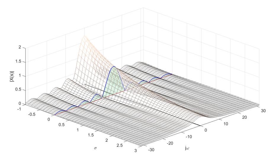
Figure 5. Visualization of $X(s)$ for the example problem. Along with it, the magnitude plot for the case where $s=j\omega$ is also shown, which represents the frequency response of the Fourier transform.
Source code: Ex 7.7, Ch 7. Laplace Transform, Signals and Systems, Oktay Alkin

If we separately plot only the $s=j\omega$ part, it would be as shown in the following figure, which is equivalent to visualizing only the magnitude of the Fourier transform of the rectangular pulse $x(t)$.

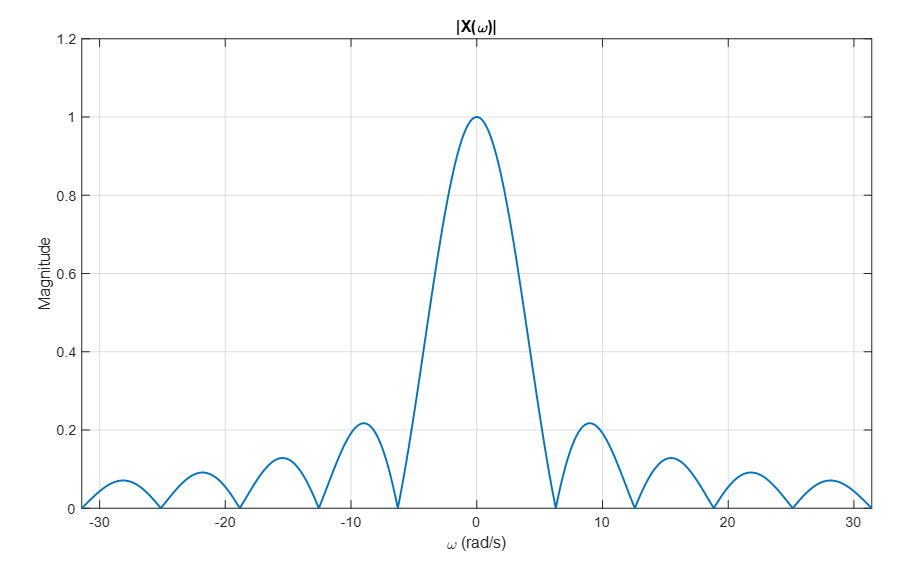
Figure 6. Visualization of the frequency response part of the Fourier transform separately
Source code: Ex 7.7, Ch 7. Laplace Transform, Signals and Systems, Oktay Alkin

Pole-Zero Plot

The result of the Laplace transform can be represented as a three-dimensional function, as shown in Figure 4 or Figure 5. However, it is almost impossible to draw such three-dimensional graphs by hand like Figure 4 or Figure 5, so information is often represented using a concept called the pole-zero plot.

When we examine the results of the Laplace transform, we often find that the magnitude of $X(s)$ diverges or becomes zero at certain $s$ points, as shown in Figure 4 or Figure 7. The most important thing in Laplace transform is not the overall shape of the three-dimensional graph, but rather where the Region of Convergence is defined, and at which $s$ values the magnitude of $X(s)$ diverges or becomes zero.

Therefore, we represent this information by drawing an “x” at the locations of $s$ where it diverges and a “o” at the locations of $s$ where it converges to zero on a two-dimensional complex plane. This graph is called a pole-zero plot.

For example, a pole-zero plot in the form of Figure 4 would look like the following:

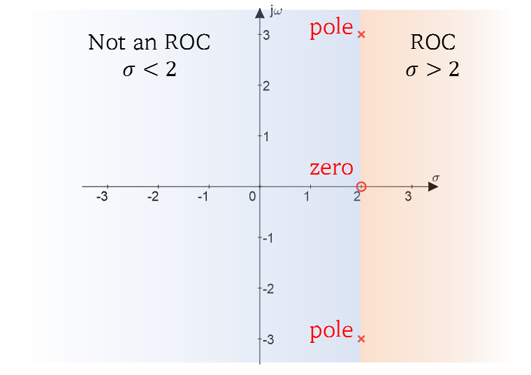
Figure 7. Pole-zero plot representing $|X(s)|$ with poles and zeros, as shown in Figure 4

In general, the result of the Laplace transform, $X(s)$, can be expressed in the following form:

\[X(s) = \frac{b_ms^m+b_{m-1}s^{m-1}+\cdots+b_1s+b_0}{a_ns^n+a_{n-1}s^{n-1}+\cdots+a_1s+a_0}\] \[=K\frac{(s-z_1)(s-z_2)\cdots(s-z_{m-1})(s-z_m)}{(s-p_1)(s-p_2)\cdots(s-p_{n-1})(s-p_n)}\]

In the above equation, $z_1, \cdots, z_m$ are called zeros, and $p_1, \cdots, p_n$ are called poles. Zeros are the values of $s$ that make $X(s)$ equal to 0, and poles are the values of $s$ that make $X(s)$ diverge to infinity.

Laplace Transform Pairs

When applying Laplace transform, it is common to match the results before and after transformation by looking at well-known transform pairs, rather than directly calculating integrals as shown in Examples 1-3 above.

Figure 8. Laplace Transform Pairs
Source: Chegg

In the above figure, there are frequently used Laplace transform pairs, so it would be helpful to use the ones needed.

Among them, we will focus on Laplace transforms related to derivative coefficients and further explore the methods for solving differential equations in the following content.

Usage of Laplace Transform for Solving Differential Equations

Among the Laplace transform pairs shown in Figure 8, there are results of Laplace transform for derivatives. In mathematical notation, they can be written as follows:

\[\frac{d}{dt}f(t) \Longleftrightarrow s\cdot F(s) - f(0^-)\]

Here, $f(0^-)$ on the right-hand side is often assumed to be 0 as the initial value of the signal $f(t)$ when solving problems. If a specific initial value is given, it is typically a constant value, so it can be easily handled without much difficulty.

Also, the Laplace transform result for the second derivative is written as follows:

\[\frac{d^2f(t)}{dt^2} \Longleftrightarrow s^2F(s)-s\cdot f(0^-)-f'(0^-)\]

If we assume that either $f(t)$ or $f’(t)$ is 0 at $t=0$, we can see that the following relationship holds regardless of the order of differentiation:

\[\frac{d^nf(t)}{dt^n} \Longleftrightarrow s^nF(s)\]

In other words, we can simplify the differential operator.

There are two main advantages of solving differential equations using Laplace transform. The first advantage is that the solution of a difficult differential equation is transformed into the form of a simple algebraic equation. The second advantage is that when using Laplace transform, we can solve non-homogeneous differential equations without separately considering homogeneous solution and particular solution. For more information on non-homogeneous differential equations, refer to the meaning of non-homogeneous differential equations post.

Example of Solving Differential Equations Using Laplace Transform

Example 1

This example is the same as the one in the meaning of non-homogeneous differential equations post, but with additional initial value conditions.

\[x''-4x'+3x=t; \quad x(0)= 0, x'(0)=0\]

Let’s take the Laplace transform of the above differential equation.

\[\mathcal{L}\lbrace x''-4x'+3x\rbrace=\mathcal{L}\lbrace t\rbrace\]

By the linearity of Laplace transform, we have

\[\Rightarrow \mathcal{L}\lbrace x''\rbrace-4\mathcal{L}\lbrace x'\rbrace+3\mathcal{L}\lbrace x\rbrace=\mathcal{L}\lbrace t\rbrace\]

Both $x(t)$ and $x’(t)$ have initial values of 0. If we denote the Laplace transform of $x(t)$ as $X(s)$, then

\[\Rightarrow s^2X(s)-4sX(s)+3X(s) = \frac{1}{s^2}\] \[=(s^2-4s+3)X(s)=\frac{1}{s^2}\] \[\Rightarrow X(s) = \frac{1}{s^2(s-1)(s-3)}\]

Let’s split the equation above into partial fractions.

\[\Rightarrow X(s) = \frac{a}{s}+\frac{b}{s^2}+\frac{c}{s-1}+\frac{d}{s-3}\]

Combining back into the original fraction,

\[\Rightarrow \frac{as(s^2-4s+3)+b(s^2-4s+3)+cs^2(s-3)+ds^2(s-1)}{s^2(s-1)(s-3)}\] \[=\frac{s^3(a+c+d)+s^2(-4a+b-3c-d)+s(3a-4b)+3b}{s^2(s-1)(s-3)}\]

Therefore, the numerator of the above equation should have a value of 1. So, first,

\[b=\frac{1}{3}\]

and let’s solve the remaining three equations simultaneously.

\[\begin{cases}a+c+d = 0 \\ -4a+1/3-3c-d = 0 \\ 3a-4\cdot(1/3) = 0\end{cases}\]

Then, we obtain the following results.

\[a=\frac{4}{9}, b = \frac{1}{3}, c = -\frac{1}{2}, d = \frac{1}{18}\]

Therefore, rewriting $X(s)$, we get

\[X(s) = \left(\frac{4}{9}\cdot\frac{1}{s}\right)+\left(\frac{1}{3}\cdot\frac{1}{s^2}\right)+\left(\left(-\frac{1}{2}\right)\cdot\frac{1}{s-1}\right)+\left(\frac{1}{18}\cdot\frac{1}{s-3}\right)\]

Taking the inverse Laplace transform of $X(s)$, we get the following.

\[x(t) = \frac{4}{9}+\frac{1}{3}t-\frac{1}{2}e^t+\frac{1}{18}e^{3t}\]

The Laplace transform pairs used for the inverse transformation are as follows.

\[\begin{cases}\mathcal{L}\lbrace u(t)\rbrace=1/s \\ \mathcal{L}\lbrace tu(t)\rbrace=1/s^2\\ \mathcal{L}\lbrace e^{at}\rbrace=1/(s-a)\end{cases}\]

Refernces

• Signals and systems, Oktay Alkin, CRC Press
• 7. Laplace transform, EEE2047S: Signals and Systems I, Fred Nicolls, University of Cape Town