Markov Chain Monte Carlo

Interactive MCMC JS Applet by Chi-Feng, Source Code

Prerequisites

To understand this post well, it is recommended to know the following:

Definition of MCMC

According to Wikipedia, Markov Chain Monte Carlo (MCMC) is “an algorithm for sampling from a probability distribution based on constructing a Markov chain that has the desired distribution as its equilibrium distribution.”

Although it may seem complicated, for now, let’s just understand that MCMC is one of the sampling methods. As always, when looking at the definition alone, it is almost impossible to understand, so we will take a closer look at each part.

In this post, we will focus on understanding the meaning of MCMC rather than conveying complex mathematical concepts.

Monte Carlo

Monte Carlo is, in short, a “simulation” performed to obtain statistical values.

The reason for performing such simulations is that, due to the nature of statistics, an infinite number of attempts must be made to know the true answer, but it is practically difficult to do so. Therefore, it makes sense to estimate the answer with a finite number of attempts.

One of the most famous Monte Carlo simulations is the calculation of the area of a circle.

As shown in the figure below, when an infinite number of points are plotted within a square with a length and width of 2, if the distance from the center is less than or equal to 1, it is colored in red, and if not, it is colored in blue.

By calculating the ratio of the total number of points plotted to the number of points colored in red and multiplying it by the area of the original square, which is 4, you can estimate the area of a circle with a radius of 1.

Figure 1. Monte Carlo simulation for approximating the area of a circle with a radius of 1

In MCMC, the name “Monte Carlo” is used to mean “trying an infinite number of something using statistical properties.”

Markov Chain

A Markov Chain is a probability process that only depends on the previous state when transitioning from one state to another.

It may sound complicated, but let’s think of an analogy:

Typically, people tend to avoid having a meal similar to the one they had the day before.

For example, if someone had Jajangmyeon (Korean black bean sauce noodles) yesterday, they would try not to have any noodle dishes today.

If today’s meal selection process only depends on yesterday’s meal selection and not on the meal selection the day before yesterday, this process has the Markov property, and this probability process can be called a Markov Chain.

As mentioned earlier, MCMC is one of the sampling methods. We can think of the word “Markov Chain” as it implies “the last selected sample recommends the next sample.”

Sampling using MCMC

MCMC is a combination of Monte Carlo and Markov Chain concepts.

In other words, performing MCMC means repeatedly attempting to recommend the next sample based on the previous one, starting with randomly selecting the first sample.

The least mathematical word in the above sentence is “recommend.”

Moreover, the process of accepting or rejecting comes after the recommendation. Let’s take a look at this process.

By the way, the MCMC sampling algorithm that we mainly introduce in this post is the Metropolis algorithm.

Sampling process (Metropolis algorithm)

First, like when performing Rejection Sampling, we need one target distribution that we want to extract samples from.

The target distribution does not necessarily have to be a probability density function. It is sufficient to use a function that is proportional to the size of the probability density function.

For example, we can use the following function as the target distribution:

\[f(x) = 0.3\exp\left(-0.2x^2\right) + 0.7\exp\left(-0.2(x-10)^2\right)\]

This function cannot be called a probability density function because the entire area from negative infinity to positive infinity is not equal to 1. However, if we know that the probability density function approximately has a similar shape to the target function $f(x)$ through experimental results, we may need sampling to approximate the actual probability density function from such a target function.

1. Random Initialization

The first step to perform in the sampling process of MCMC is random initialization. Simply put, it means selecting any input value in the sample space. For example, we can choose $x_0$ randomly, as shown in the figure below. In this case, $x_0$ is set to 7. This is an arbitrary starting point to begin the MCMC algorithm, unrelated to the target distribution.

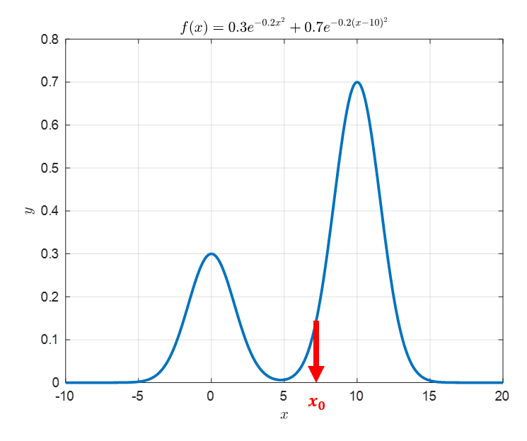
Figure 2. Select an arbitrary starting point to begin the MCMC algorithm, unrelated to the target distribution.

2. Obtaining the Next Point from the Proposal Distribution

The next step in MCMC is to obtain a recommendation for the next sample to extract from the proposal distribution. Any probability distribution can be used as the proposal distribution, but Metropolis proposed an algorithm for the case of using a symmetric probability distribution, and Hastings extended the algorithm proposed by Metropolis to the case of using a general probability distribution. For simplicity, let’s use a symmetric probability distribution as the proposal distribution, which we will call $g(x)$.

The commonly used symmetric proposal distribution is the normal distribution, which can be centered around the initially chosen $x_0$. The width of the normal distribution (i.e., standard deviation) can be arbitrarily set by the researcher. In this example, we set the standard deviation to 2.

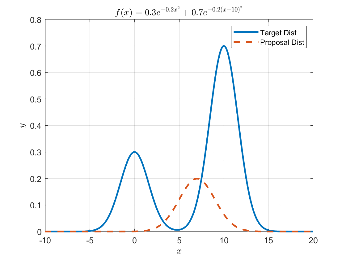
Figure 3. Form the proposal distribution centered at the starting point.

It is easy to extract samples from this normal distribution, which has a mean of 7 and a standard deviation of 2. In MATLAB, we can use the randn() function to easily extract samples.

Let’s consider recommending the next point from the proposed distribution as shown below.

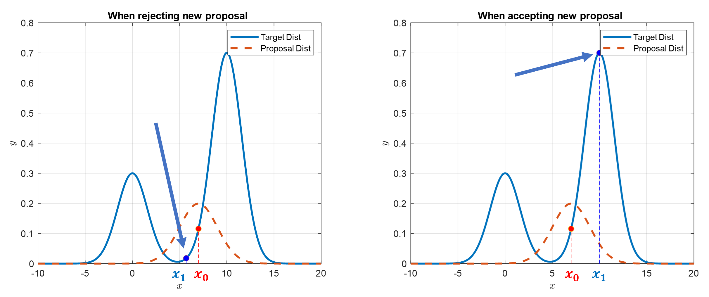
Figure 4. The blue dots represent newly proposed sample points and the values of the target distribution at those points.

In Figure 4, the blue dots represent newly proposed sample points and the values of the target distribution at those points.

Also, if we look closely at Figure 4, the newly proposed sample point on the left side of the figure is rejected while the one on the right side is accepted.

The reason for rejection is that the height of the target distribution at the proposed sample point is lower than the height at the original $x_0$.

On the other hand, the reason for acceptance is that the height of the target distribution at the proposed sample point is higher than the height at the original $x_0$.

In other words, acceptance is determined based on the following criterion:

\[\frac{f(x_1)}{f(x_0)}>1\]

If the proposal is accepted, the proposed distribution is drawn around the accepted sample point and a new sample is recommended based on this distribution.

However, if the proposal is rejected, MCMC has a way to statistically accept rejected samples, called “consolation match”.

3. Consolation Match

The rejected samples from step 2 are not completely discarded, but rather can be statistically accepted.

Let’s assume the original sample position is $x_0$, and the newly proposed sample position from the proposal distribution is $x_1$.

Then, if the target distribution is denoted as $f(x)$ as before, we check the following:

For a randomly sampled $u$ from the uniform distribution $U_{(0,1)}$,

\[\frac{f(x_1)}{f(x_0)}>u\]

If the above inequality is satisfied, the sample is accepted even if the target distribution height for the new sample is not higher.

If the inequality is not satisfied, the new sample $x_1$ is rejected, and the next sample ($x_2$) is recommended with $x_0$ as the new sample.

This process is repeated for steps 2-3.

Pseudo-code of the algorithm

This is the end of the MCMC algorithm. It’s really simple.

If we write this content in pseudo-code, it looks like this:

Initialize $x_0$

For $i=0$ to $N-1$

Sample $u\sim U_{[0,1])}$

Sample $x_{new}~g(x_{new}|x_i))$

If $u\lt A(x_i, x_{new}) = min\left\lbrace 1, f(x_{new})/f(x_i)\right\rbrace$

$\quad x_{i+1} = x_{new}$

else

$\quad x_{i+1} = x_i$

What if the proposal distribution is not symmetric?

In the case where the proposal distribution is not symmetric, we can use the Metropolis-Hastings algorithm, an upgrade of the Metropolis algorithm for this purpose.

In the Metropolis-Hastings algorithm, when comparing the likelihood of the target distribution shown in equation (2), we also need to use the height of the proposal distribution to adjust the value.

In other words, the criterion in equation (2) can be adjusted as follows:

If we denote the proposal distribution as $g(x)$, then

\[\text{Equation (2)} \Rightarrow \frac{f(x_1)/g(x_1|x_0)}{f(x_0)/g(x_0|x_1)}\]

In other words, in the numerator of equation (4), we normalize the new point $x_1$ using the value $g(x_1|x_0)$, which is drawn based on $x_0$. Similarly, in the denominator, we normalize the previous point $x_0$ using the value $g(x_0|x_1)$, which is drawn based on the new point $x_1$.

Pseudo-code of the algorithm

This is the end of the MCMC algorithm. It’s really simple.

If we write this content in pseudo-code, it looks like this:

Initialize $x_0$

For $i=0$ to $N-1$

Sample $u\sim U_{[0,1])}$

Sample $x_{new}~g(x_{new}|x_i))$

If $u\lt A(x_i, x_{new}) = min\left\lbrace 1, f(x_{new})/f(x_i)\right\rbrace$

$\quad x_{i+1} = x_{new}$

else

$\quad x_{i+1} = x_i$

What if the proposal distribution is not symmetric?

In the case where the proposal distribution is not symmetric, we can use the Metropolis-Hastings algorithm, an upgrade of the Metropolis algorithm for this purpose.

In the Metropolis-Hastings algorithm, when comparing the likelihood of the target distribution shown in equation (2), we also need to use the height of the proposal distribution to adjust the value.

In other words, the criterion in equation (2) can be adjusted as follows:

If we denote the proposal distribution as $g(x)$, then

\[\text{Equation (2)} \Rightarrow \frac{f(x_1)/g(x_1|x_0)}{f(x_0)/g(x_0|x_1)}\]

Bayesian Estimation using MCMC

MCMC can be used not only for sampling but also for parameter estimation.

Prerequisites

To better understand this content, it is recommended that you have knowledge of the following:

What is given?

Let’s try to perform parameter estimation using MCMC.

For example, let’s say we were able to extract 1,000 samples from a population of 30,000 elements that follows a normal distribution with a mean of 10 and a standard deviation of 3.

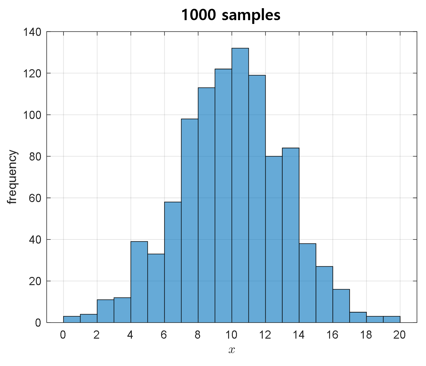
Figure 6. 1,000 samples prepared for Bayesian estimation

What we want to know is how to better estimate the mean value of the entire population of 30,000 using only these 1,000 samples.

Estimation process

1. Random Initialization

Just like in the sampling process of MCMC, random initialization is used to start the MCMC algorithm in parameter estimation.

Assuming that we know that the probability density function of the population we want to estimate follows a normal distribution, we can try to estimate two parameters, the mean and the standard deviation.

However, for the sake of explanation, we will only estimate the mean value and use the sample standard deviation as it is.

First, let’s initialize randomly, which is the principle, but starting from a mean value of 1, let’s see if the estimated value approaches the true value of 10.

The sample standard deviation of the 1,000 samples is calculated to be 3.1591.

Therefore, our target distribution is a Gaussian distribution, and the standard deviation will continue to be fixed at 3.1591 as we move forward.

2. Propose a new mean value using a proposal distribution

Let’s use an algorithm that is used in MCMC using a proposal distribution to recommend a new mean value through the proposal process.

To do this, let’s draw a proposal distribution centered around the initialized mean value of 1 in the same way as the sampling process.

Any distribution can be used as a proposal distribution, but for the sake of convenience in the discussion, let’s use a symmetric probability distribution, such as the normal distribution.

The normal distribution with a standard deviation of 0.5 will be used as the proposal distribution.

Then, we can recommend a new mean value by sampling from this proposal distribution.

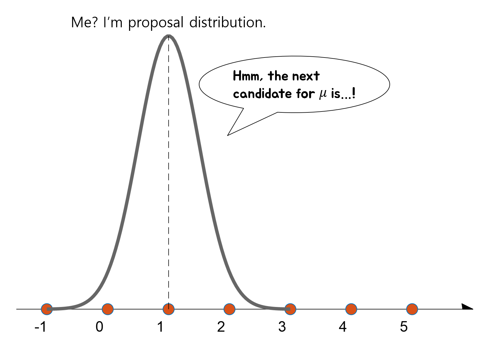
Figure 7. A new $\mu$ can be recommended by sampling a new sample from the proposal distribution with $\mu=\mu_{old}$ as the center.

3. Acceptance or rejection of the proposed value

※ From here on, Bayes’ theorem is introduced and the equations become more complicated, but even if you only know the result of the final equation (13), it is not difficult to understand MCMC. ※

Now we need to accept or reject the recommended mean value.

Acceptance or rejection can be done by comparing the height of the target function, just like in the previous sampling method.

However, the difference this time is that we are comparing the two cases where the target function’s parameter has changed. Why do we compare the two cases where the parameter has changed? It’s because what we want to do now is parameter estimation, and in parameter estimation, we need to confirm whether the current parameter (mean in this case) is better than the previous parameter.

In other words, comparison is made based on the following formula. If this comparison criterion is satisfied, the proposal is accepted, and if not, it is rejected.

\[Criterion: \frac{f_{new}(x)}{f_{old}(x)} > 1\]

The formula (5) can also be rewritten as follows:

\[\frac{P(\theta = \theta_{new}|Data)}{P(\theta = \theta_{old}|Data)}>1\]

In equation (6), $Data$ can be considered as the 1,000 samples seen in Figure 6.

Here, according to Bayes’ theorem, equation (6) can be transformed as follows:

\[\frac{f(D|\theta=\theta_{new})P(\theta=\theta_{new})/f(D)}{f(D|\theta=\theta_{old})P(\theta=\theta_{old})/f(D)}>1\]

In equation (7), since $f(D)$ is the same in the numerator and denominator, it can be removed, resulting in the following:

\[Equation(7) \Rightarrow \frac{f(D|\theta=\theta_{new})P(\theta=\theta_{new})}{f(D|\theta=\theta_{old})P(\theta=\theta_{old})}>1\]

The terms related to $f(D|\theta)$ in the numerator or denominator all represent the likelihood of the entire dataset. Assuming that all data are independently obtained, they can be expressed for each data point $d_i$ as follows:

\[f(D|\theta) = \prod_{i=1}^N f(d_i|\theta)\]

Here, $N$ is the total number of data points, and each data point is denoted as $d_i$.

Since our target distribution is a normal distribution,

\[Equation(9)\Rightarrow \prod_{i=1}^{N}\frac{1}{\sigma\sqrt{2\pi}}\exp\left(-\frac{(d_i-\mu)^2}{2\sigma^2}\right)\]

To facilitate calculation, let’s take the natural logarithm of equation (10):

\[\Rightarrow \sum_{i=1}^{N}\left\lbrace\log\left(\frac{1}{\sigma\sqrt{2\pi}}\right)-\frac{(d_i-\mu)^2}{2\sigma^2}\right\rbrace\] \[=\sum_{i=1}^{N}\left\lbrace-\log(\sigma\sqrt{2\pi})-\frac{(d_i-\mu)^2}{2\sigma^2}\right\rbrace\]

Now, taking the natural logarithm of the original equation (8) and substituting equation (12), we get:

\[Equation(8)\Rightarrow \frac{\sum_{i=1}^{N}\left\lbrace-\log(\sigma\sqrt{2\pi})-\frac{(d_i-\mu_{new})^2}{2\sigma^2}\right\rbrace + \log(P(\mu = \mu_{new}))}{\sum_{i=1}^{N}\left\lbrace-\log(\sigma\sqrt{2\pi})-\frac{(d_i-\mu_{old})^2}{2\sigma^2}\right\rbrace + \log(P(\mu = \mu_{old}))} > 1\]

So, what does equation (13) mean?

We can see that it is a comparison of the likelihood times prior for the cases where $\mu=\mu_{old}$ and $\mu=\mu_{new}$, given the given data.

Figure 8 below shows the process of obtaining likelihood values from all data for the target distribution in the case of $\mu=\mu_{old}$ and $\mu=\mu_{new}$.

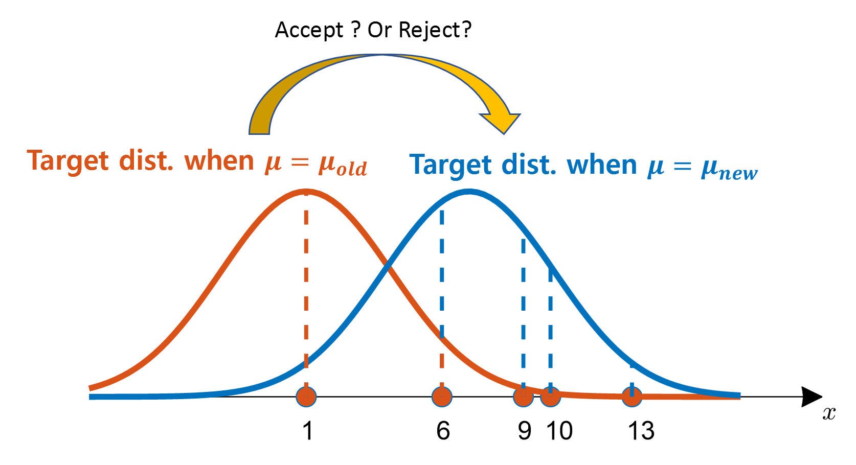
Figure 8. The process of multiplying the likelihood of all data for the cases of $\mu=\mu_{old}$ and $\mu=\mu_{new}$

Although only five data points are shown in Figure 8, there are more data points with higher likelihood (the height of the probability density function) for the case of $\mu=\mu_{new}$ than for the case of $\mu=\mu_{old}$, because $\mu=\mu_{new}$ is closer to the actual population mean value (10). After multiplying all the likelihoods and comparing them with the prior, the recommendation of $\mu=\mu_{new}$ can be adopted.

Now, looking at equation (13), since $\sigma$, $\mu_{new}$, and $\mu_{old}$ are all given, there is no problem with calculating them. However, how do we calculate priors such as $P(\mu=\mu_{new})$ and $P(\mu=\mu_{old})$?

As I explained in the post on the meaning of Bayes’ theorem or the post on naive Bayes classifiers, priors are a kind of prior knowledge, and even if they are very small, we can input information about $\mu$ values.

Here, using the prior knowledge that we can roughly infer from looking at Figure 6, the value of $\mu$ we want to estimate is at least greater than 0. Therefore, we can set the prior as follows:

\[P(\mu) = \begin{cases}1 && \text{if }\mu\gt 0 \\ 0 && \text{otherwise}\end{cases}\]

If you are more confident, you can use a better condition than the condition that it is greater than 0, such as that it is greater than 3.

In any case, we will adopt the newly recommended $\mu_{new}$ when equation (13) is satisfied, and reject it if it is not.

However, as with the sampling method, we can go through a consolation match if equation (13) is not satisfied.

4. Consolation Match

If equation (13) is not satisfied, we can go through a consolation match, as with the sampling method.

In this case, we can accept $\mu_{new}$ if the following equation is satisfied for a value of $u$ extracted from the uniform distribution $U_{[0, 1]}$ with an interval of $[0, 1]$:

\[\frac{\sum_{i=1}^{N}\left\lbrace-\log(\sigma\sqrt{2\pi})-\frac{(d_i-\mu_{new})^2}{2\sigma^2}\right\rbrace + \log(P(\mu = \mu_{new}))}{\sum_{i=1}^{N}\left\lbrace-\log(\sigma\sqrt{2\pi})-\frac{(d_i-\mu_{old})^2}{2\sigma^2}\right\rbrace + \log(P(\mu = \mu_{old}))} > u \notag\] \[\text{where } u \sim U_{[0, 1]}\]

Results of the estimation

As shown in Figure 9, we can see that starting from an initial value of $\mu = 1$, the estimate gradually approaches the true population mean of 10 as the iterations progress. It can also be seen that after about 20 iterations, the estimate starts to fluctuate around the true population mean.

This initial period of iterations that is required to converge to the true population mean is commonly referred to as the burn-in period.

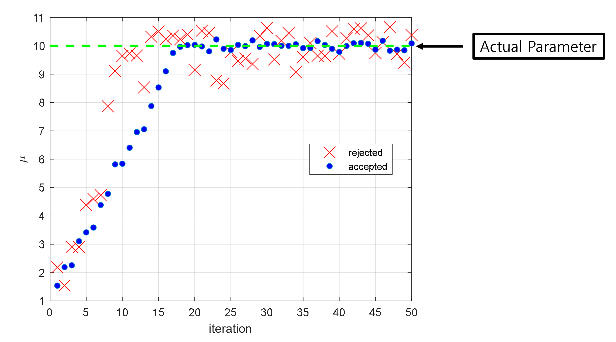
Figure 9. Accepted or rejected $\mu$ values during the first 50 iterations

Figure 10 shows the $\mu$ values that were accepted or rejected during 12,000 iterations.

In Figure 10, we can see that when the estimate is far from the true population mean of 10, it is rejected, but when the estimate is close to the true population mean, it is accepted.

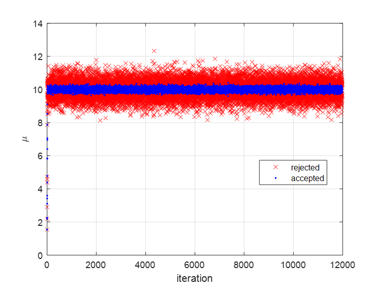
Figure 10. Accepted or rejected $\mu$ values during the entire 12,000 iterations

By taking the first 25% of the iterations as the burn-in period and averaging all the accepted $\mu$ values during the remaining 75% of the iterations, we found that the estimated population mean is 9.99, which is very close to the true population mean of 10.

Using this estimated population mean of 9.99, we can estimate the population distribution, which is very similar to the original population distribution as shown in Figure 11.

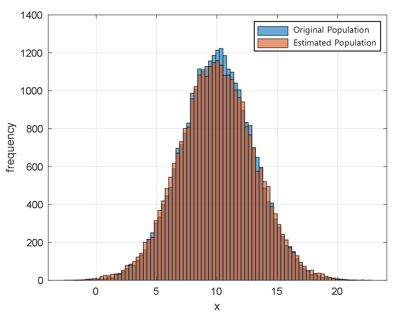
Figure 11. Population distribution estimated using the estimated $\mu$ value and the original population distribution