※ The Wilcoxon rank sum test is equivalent to the Mann-Whitney U test.
※ The contents of this posting were written with reference to Stanton Glantz’s Primer of biostatistics textbook.
Prerequisites
To better understand this posting, it is recommended to have a good understanding of the following.
Motivation
The parametric statistical methods such as t-test or ANOVA are based on the following assumptions:
“The sample data are extracted from a population with a normal distribution, and although the mean value changes due to the treatment, the variance does not change.”
In many cases, it can be assumed that the sample data is extracted from a normal distribution, and if the sample size is large, the sample mean follows a normal distribution (because of the central limit theorem), so the above assumption is often valid. This is why t-tests and ANOVA are widely used statistical techniques.
However, if the data does not satisfy this assumption, it is not possible to use parametric tests and nonparametric tests should be used. In other words, when it is difficult to be sure that the population distribution is a normal distribution or when the number of data samples is too small, it is worth considering using a nonparametric test. Also, if only ranks are obtained and not continuous numerical values when measuring data, nonparametric tests should be considered because it is not possible to use parametric tests.
In this chapter, we will learn about the Wilcoxon rank sum test, which is known to replace independent t-test. In other words, we will learn about techniques for statistically comparing two independently extracted sample groups without assuming normality.
Rank sum test
Introduction to the principle of the rank sum test
The rank sum test is not substantially different from the t-test in principle. Let’s recall how we thought about the distribution of t-values in The Meaning of t-Value and Student’s t-Test.
First, we defined the t-value statistic, and then we simulated the distribution of t-values that could be extracted from the population for two sample groups selected randomly.
The figure below shows the simulation of the t-value distribution by repeatedly selecting two samples of n=6 from a population of 150 100 times.
Figure 1. The distribution of t-values obtained every time by extracting two sample groups with n=6 a hundred times
The rank sum test is not significantly different from this process. First, we define a statistic that plays the same role as the t-value above, and then we will confirm the distribution of all possible statistics that can be obtained through simulation.
We then check how significant the two sample groups we have are really different by checking how large the statistic value of the given data is.
The figure below is an example data given to us. This data is virtual experimental data to see the effect of a diuretic. (Source: S. Glantz’s book, Primer of Biostatistics)
The data is divided into two groups, one group who received a placebo and the other group who received a diuretic.
There are a total of three people in the placebo group and four people in the diuretic group, and the urine volume of each subject is indicated.
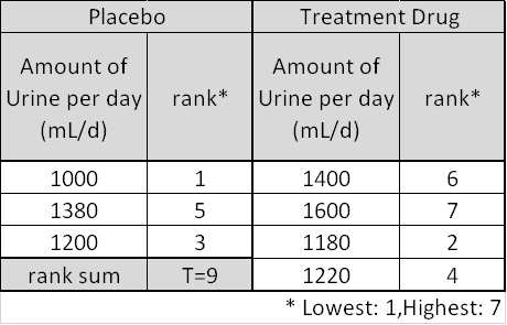
Figure 2. Example data to explain the rank sum test. Experimental data on the intake of diuretics.
Source: Primer of Biostatistics, 7th ed., S. Glantz
Looking at this data, we can see that the sample size within the group is very limited. Therefore, it can also be seen as a case where non-parametric tests can be performed as the sample size is small.
To perform nonparametric tests, especially rank-based tests, the first thing to do is to calculate the rank of the data using the value of each data. Here, we calculated the rankings by setting the data with the smallest value as rank 1 and the data with the largest value as rank 7.
(Even if you rank the data in reverse order, with the smallest value being ranked 7 and the largest value being ranked 1, it does not affect the analysis results.)
Then, as shown in Figure 2, let’s calculate a statistic called the “sum of ranks”.
As shown in the left side of Figure 2, the placebo group has a total sum of ranks T equal to 9.
So, the problem we face here is as follows:
"Can we say that this value of T=9 is small enough?"
Now, as we considered the t-distribution in the meaning of t-value and Student’s t-test, we can also check the distribution of the sum of ranks statistic T.
If we only consider the number of cases where three out of the seven ranks (1-7) are chosen, we can know the distribution of all possible values of the sum of ranks statistic T.
Therefore, as shown in Figure 3 below, let’s consider all possible cases where three out of the seven ranks are selected, and calculate the corresponding sum of ranks statistic T for each case.
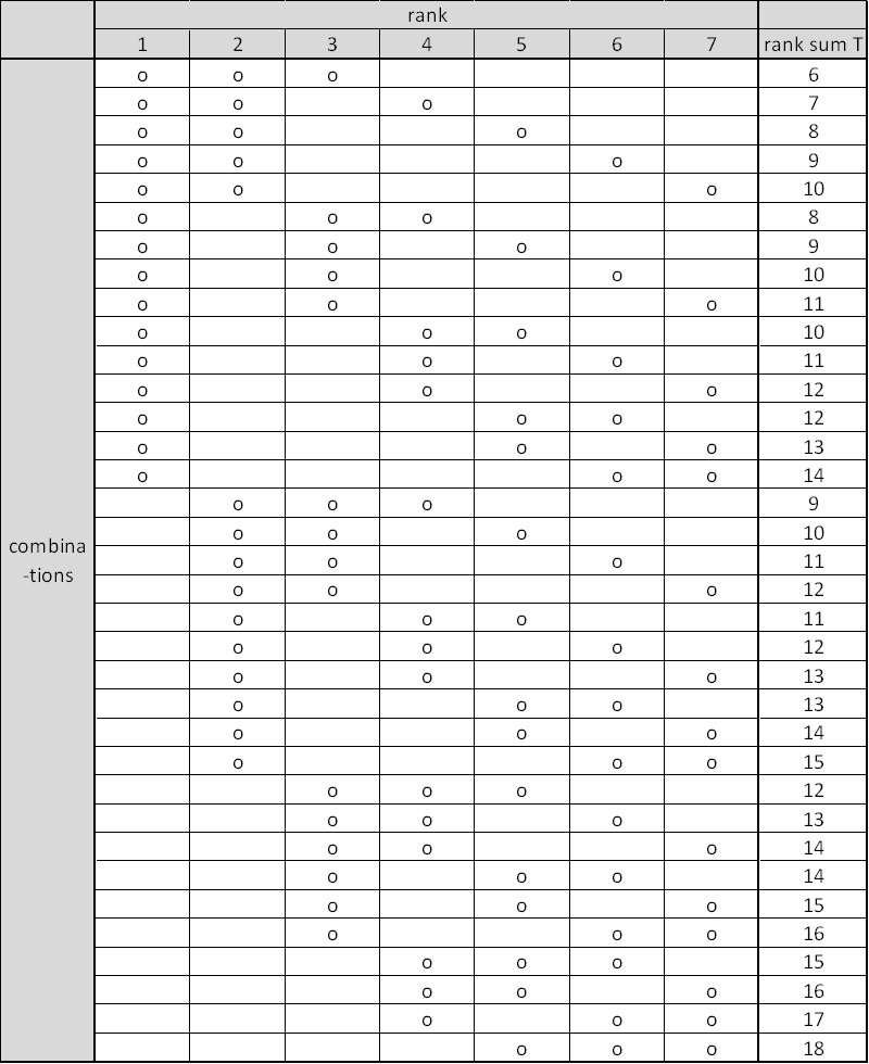
Figure 3. The number of cases where three out of the seven ranks are selected and the corresponding sum of ranks statistic T for each case.
For example, the first row assumes that the data ranked 1st, 2nd, and 3rd are from the placebo group, and the sum of ranks statistic T in this case is 6.
Once the sum of ranks statistic T for all possible cases is examined as shown in Figure 3, let’s draw a histogram of the sum of ranks statistic T for all possible values.
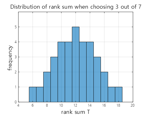
Figure 4. The histogram of the sum of ranks statistic T for all possible combinations.
When looking at this, we can see that the most extreme cases are when $T=6$ or $T=18$, and even these are the first or last cases out of a total of 35 cases, so the probability of obtaining a $T$ value that corresponds to $T=6$ or $T=18$ by chance (i.e., the p-value) when the treatment drug has no effect is
\[2\times \frac{1}{35} = 0.057\](since we are conducting a two-sided test).
Therefore, we can conclude that the $T$ value of 9 from our available data is a case that is difficult to show a difference between the two groups.
One thing to note is that all possible values of $T$ that can be obtained are combinations of rankings, so they can only be discrete, and the p-value may not come out as a continuous value.
The following table summarizes the significant rank sum statistics $T$ according to the experimental conditions. $n_S$ represents the number of samples in the group with fewer samples, and $n_B$ represents the number of samples in the group with more samples.
Also, we have listed the $p$-values that are most commonly used in parametric methods, $p=0.05$ and $p=0.01$, as well as the $p$-value that is closest to them.
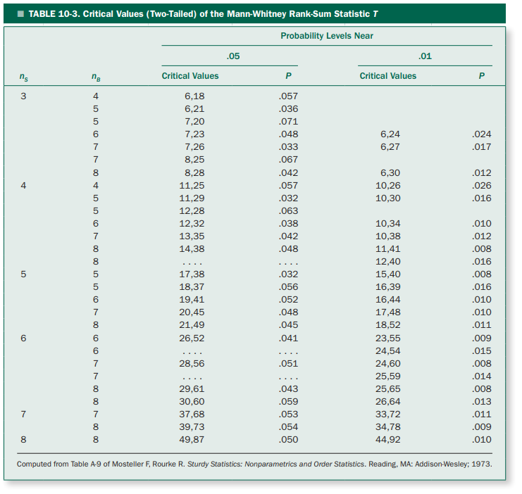
Figure 5. Significant rank sum statistics $T$ and their corresponding p-values according to the experimental conditions
Source: Primer of Biostatistics, 7th ed., S. Glantz
Normal approximation of rank-sum test
During analysis, there may be times when non-parametric tests need to be used even when there are a large number of samples.
For example, suppose there are 10 samples in each of two groups. In this case, the number of ways to select 10 out of 20 ranks is
\[_{20}C_{10}=184,756\]which makes it difficult to write everything down in a table. Therefore, in such cases, a normal approximation is used. It is known that if one group has at least 8 samples, the distribution of T can be approximated by a normal distribution with the following mean and standard deviation:
\[\mu_T=\frac{n_S(n_S + n_B + 1)}{2}\] \[\sigma_T=\sqrt{ \frac{n_Sn_B(n_S+n_B+1)}{12} }\]Therefore, if we express T as the following test statistic $z_T$, it is possible to perform a test for the normal distribution.
\[z_T = \frac{T-\mu_T}{\sigma_T}\]There is a process called continuous correction that can be applied to correct the discrete error that occurs when aligning the distribution of T with a continuous distribution such as z, since the distribution of T is discrete.
\[\Rightarrow z_T = \frac{ \left| T-\mu_T \right|-1/2 }{ \sigma_T }\]Reference
- Primer of biostatistics, 7th ed., S. Glantz / Ch. 10 Alternatives to Analysis of Variance and the t Test Based on Ranks