“Divergence” and “Curl” are operators applied in vector fields. First of all, a vector field can be defined as a correspondence between points in Euclidean space and vectors.
They are used to represent the magnitude and direction at each point of phenomena such as fluid flow and gravitational fields. (Wikipedia, Vector field)
Divergence
Divergence is an operator that measures the extent to which a vector field spreads out or converges to a point $(x,y)$ within a very small region in the vector field.
Although it may be insufficient, one way to think about it is as the normalized change in the direction towards which the vector field is pointing at the arbitrary point $(x,y)$.
Physically, divergence of a vector field can be thought of as the amount of flow per unit volume that enters or leaves and changes within a very small region (infinitesimal area or volume).
Before examining whether the vector field spreads out within a very small region, let’s first check if the vector field emerges or converges to a point at a more macro scale.
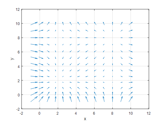
Figure 1. Vector field with points where it converges or emerges on the xy-plane
Let’s consider a vector field on the xy-plane as shown above. Upon closer inspection, you may notice that there are points at (2,2), (2,8), (8,2), and (8,8) where the vector field converges or emerges.
Then, how can we think about the amount of divergence at an arbitrary point at a macro level? In general, we can think about it as follows.
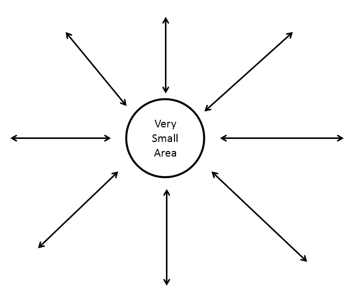
Figure 2. How to think about the amount of divergence at a macro level
However, in order to define the divergence in this way, there are issues to consider.
The biggest problem is that the arrows depicted in Figure 2 actually show a few sampled vectors from within the vector field, but in reality, there are a very large number of vectors entering or leaving a ‘relatively small region’. Therefore, when considering the divergence, we need to consider the divergence of vectors in the infinitesimal region.
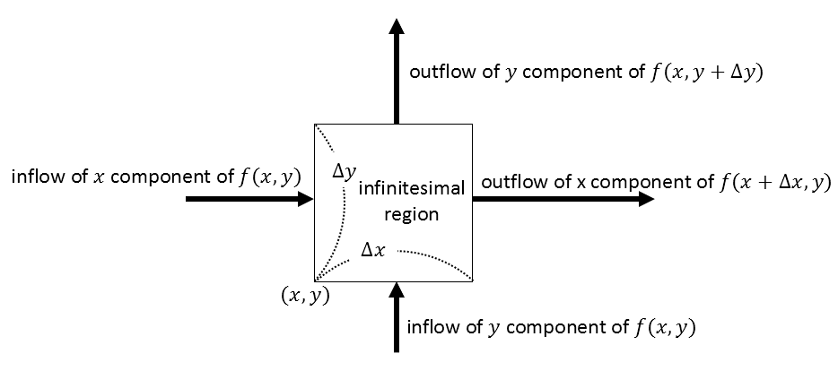
Figure 3: Divergence of vector field in infinitesimal region
By considering only the difference between the inflow and outflow of vectors in the infinitesimal region, we can only consider the vectors entering or leaving from two directions, as it is the limit of the region.
Then, how can we determine the divergence of vectors in the infinitesimal region?
It is given by the formula (Outflow - Inflow). Of course, we need to combine the divergence in the $x$-direction and the $y$-direction.
So, if we define the vector function $f(x, y)$ as $f(x, y) = P(x, y)\hat{i} + Q(x, y)\hat{j}$, the divergence in the infinitesimal region can be defined as follows:
Divergence in infinitesimal region = Divergence in $x$-component direction + Divergence in $y$-component direction
\[= \lim_{\Delta x\rightarrow 0}\lim_{\Delta y\rightarrow 0} \left\{ \frac{P(x+\Delta x, y+\frac{1}{2}\Delta y) - P(x, y+\frac{1}{2}\Delta y)}{\Delta x} + \frac{Q(x+\frac{1}{2}\Delta x, y+\Delta y) - Q(x+\frac{1}{2}\Delta x, y)}{\Delta y} \right\}\]Dividing by $\Delta x$ and $\Delta y$ normalizes the divergence according to the width and height of the infinitesimal region.
Therefore, the divergence in the infinitesimal region can also be expressed using the definition of partial derivatives:
\[\text{Divergence in infinitesimal region} = \frac{\partial P}{\partial x} + \frac{\partial Q}{\partial y}\]On a side note, if you have studied scalar fields and gradients, you may have come across the Del operator. For review purposes, the gradient of a scalar function (or field) is expressed as follows: [insert gradient formula]
\[gradient(f) = \nabla f=\frac{\partial}{\partial x}f(x,y)\hat{i} + \frac{\partial}{\partial y}f(x,y)\hat{j}\]We can separate the $\nabla$ operator as follows:
\[\nabla = \frac{\partial}{\partial x}\hat{i} +\frac{\partial}{\partial y}\hat{j}\]The divergence of a vector, according to my definition, can be thought of as measuring the rate of change of the vector field in the direction it points, obtained by taking the dot product of $\nabla$ and the vector field $f(x,y)$.
Let’s denote the vector field $f(x,y)$ as $P(x,y)\hat{i}+Q(x,y)\hat{j}$. The divergence of the vector field $f$ can be calculated as follows:
\[\nabla \cdot f = \left(\frac{\partial }{\partial x}\hat{i} + \frac{\partial }{\partial y}\hat{j}\right)\cdot\left(P(x,y)\hat{i} + Q(x,y)\hat{j}\right) = \frac{\partial P}{\partial x} + \frac{\partial Q}{\partial y}\]This is equivalent to the amount of flux through the infinitesimal region calculated earlier.
It should be noted that divergence is applied to a vector field and results in a scalar value at any arbitrary point $(x,y)$.
Example of Divergence
Now, let’s consider a vector field as an example:
\[f(x,y) = 2x\hat{i} + (0)\hat{j}\]In other words, it is a vector field that increases in magnitude as it moves towards the positive x-axis, but still points to the right. If we plot this vector field using MATLAB, we get the following:
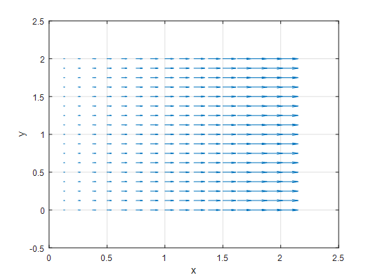
Figure 4. Plot of the vector field $f(x,y)=2x\hat{i}$
So, what does the divergence of this vector field mean? Let’s calculate the divergence:
\[\nabla \cdot f = \frac{\partial (2x)}{\partial x} + \frac{\partial(0)}{\partial y} = 2\]The divergence of this vector field is always 2, regardless of the point on the $xy$-plane. What does this mean?
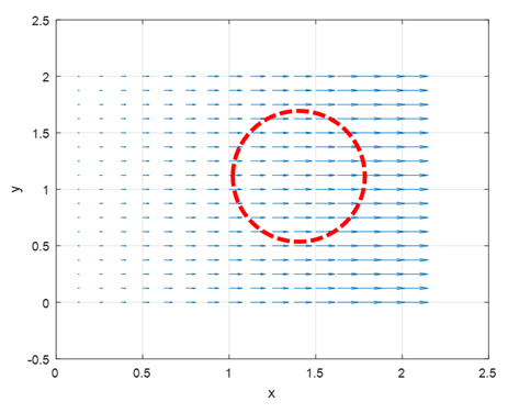
Figure 5. Let's set an arbitrary region on the vector field. The red region indicates an arbitrary area. What is the net sum of the vectors entering and leaving the region?
Let’s take a look at Figure 5. It shows a vector field $f(x, y) = 2x\hat{i}$, and on top of it, we have drawn an arbitrary region with a red circle. You can see that there are vectors entering and leaving this circle.
In this case, the net sum of the entering and leaving vectors is positive.
As the circle becomes smaller and approaches a infinitesimal area, the change in the net sum of normalized vectors is 2.
This means that the net sum of vectors changes with a rate of 2, indicating a change in velocity.
Divergence can be thought of as obtaining the acceleration at each arbitrary point $(x, y)$ when applied to a vector field with velocity vectors.
Now let’s examine the divergence of the vector field in Figure 1.
The vector field in Figure 1 is given by the following vector function:
\[f(x, y) = (x-2)(x-8)\hat{i} + (y-2)(y-8)\hat{j}\]Calculating the divergence, we get:
\[\nabla \cdot f = 2x-10+2y-10 = 2x+2y-20\]This means that above the line $y=-x+10$, the divergence value is positive, and below the line, the divergence value is negative.
If we verify this using MATLAB, we can see that the results match exactly with the calculated values.
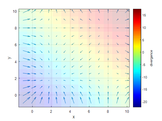
Figure 6: Plot of the divergence of $f(x) = (x-2)(x-8)\hat{i} + (y-2)(y-8)\hat{j}$. Above the line $y=-x+10$ has positive divergence, and below the line has negative divergence values.