Prerequisites
To understand the content of this post, it is recommended that you have knowledge of the following:
From Regression to Classification…
The data used in the Linear Regression (Optimization Perspective) post had continuous label values (i.e., the number of car accidents in Figure 1 below).
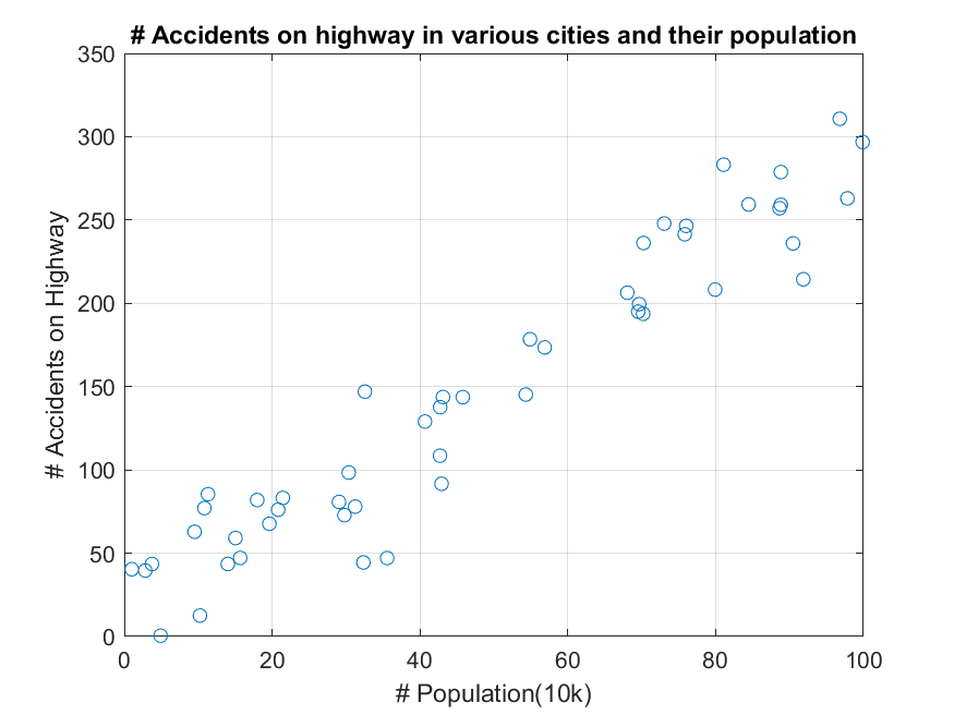
Figure 1. Data with continuous labels used in building a linear regression model.
However, in some cases, the label may be categorical. Categorical labels refer to data that cannot be represented by continuous numbers, such as “male/female” or “dog/cat”, and are usually converted to numbers such as 0 or 1.
For example, consider a case where if the value of a feature called $x$ is less than 5, the class is determined to be 0, and if it is greater than or equal to 5, the class is determined to be 1.
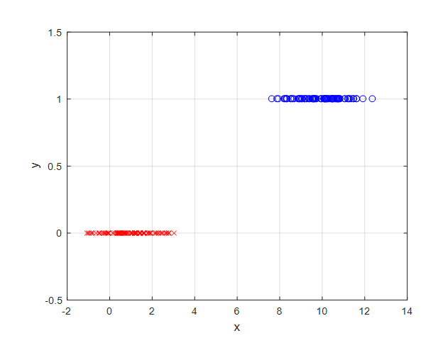
Figure 2. An example of categorical data. Let's assume that if the feature value $x$ is less than 5, the class is 0, and if it is greater than or equal to 5, the class is 1.
However, if linear regression is applied to data with categorical labels like this, the following result will be obtained:
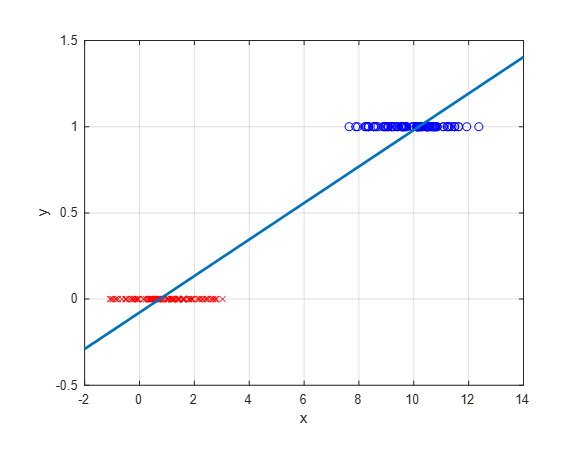
Figure 3. Applying linear regression to categorical data.
Even when applying linear regression, we can classify 1 if $\hat{y} = ax+b\geq 0.5$ and 0 otherwise.
However, for data with categorical labels, a better result can be obtained by using the following function if we perform regression analysis.
In other words, let’s think about a model that is more suitable for categorical data than a linear model.
To build a model for categorical data, we need a function that has a value of 0 before crossing a certain threshold and a value of 1 after crossing it, as shown in Figure 4 below.
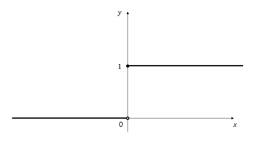
Figure 4. The form of the function that suits categorical data should be a curve that outputs 0 before a certain $x$ value and 1 after that value.
There could be several candidates for the S-shaped curve function, but let’s use the sigmoid function.
The sigmoid function is written as follows:
\[S(x) = \frac{1}{1+\exp(-x)}\]Although other functions can be used besides the sigmoid function, we choose to use it because we assume that the distribution of each class of independent variable $x$ follows a normal distribution, which will be discussed later.
Anyway, the shape of the sigmoid function is as follows:
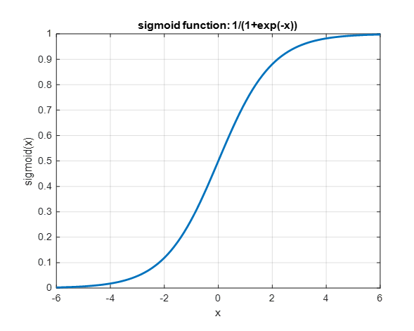
Figure 5. The shape of the sigmoid function.
When the output of this sigmoid function is greater than 0.5, we can think of the label as 1, and when it is not, we can think of it as 0.
If we apply the sigmoid function to our data shown in Figure 2, the resulting regression model will have the form of Figure 6 below:
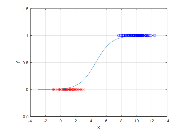
Figure 6. An example of a regression model created using the sigmoid function.
To determine the shape of the sigmoid function, we can put the parameters $a$ and $b$ into the equation of the sigmoid function as follows:
\[S(x) = \frac{1}{\exp(-(ax+b))}\]If we think carefully about this form, it can also be seen as a form in which $ax+b$ is inputted into a specific function.
The value of $b$ will play a role in shifting the sigmoid function to the left or right, while the value of $a$ will determine the steepness of the sigmoid function.
Please move the sliders ^^
In any case, we need to determine the values of $a$ and $b$, and as with building a model using linear regression, we can determine $a$ and $b$ by defining the error and minimizing this error.
Defining the error function
Now that we have determined the model, we can define the error and determine the parameters by minimizing it.
The problem we are currently considering is binary classification, where the output is either 0 or 1.
There is a slight difference from the regression model we dealt with in linear regression, in that in classification problems, the answer is either correct or incorrect.
Therefore, when we get the answer right, let’s set the error value to 0, and when we get the answer wrong, let’s set the error value to be as large as possible.
Let’s call the result we get from our equation (2) $P$. We can name it $P$ because it can be considered as the probability value for the label. For example, if $P$ is greater than or equal to 0.5, we will predict the label for this data as 1, otherwise we will predict the label as 0.
In other words, our model’s output function is as follows:
\[P = \frac{1}{1+\exp(-(ax+b))}\]That is, what we want is that when the original label $y$ is 1, if the value of $P$ is 0, we will give a large error value, and when the label $y$ is 0, if the value of $P$ is 1, we will give a large error value.
We can use the logarithmic function for this, since the form of the logarithmic function is:
\[\begin{cases}\lim_{x\rightarrow 0^+}\log(x) = -\infty \\\log(1) = 0\end{cases}\]In other words, we can think of our error as follows:
\[E(y, P) = \begin{cases}-\log(P) &&\text{ if } y = 1 \\ -\log(1-P) &&\text{ if }y = 0\end{cases}\]If we consider equation (5) carefully, when $y=1$, the error will output an infinitely large value if $P$ is output as 0, but the error will be 0 if $P$ is output as 1. Conversely, when $y=0$, if $P$ is output as 0, $-\log(1-P)$ will be $\log(1)$, which is 0, but the error will be infinitely large if $P$ is output as 1. Since $y$ can only have the values 0 or 1 due to the nature of classification, equation (5) can be written in a single line as follows:
\[E(y, P) = -(y\log(P)+(1-y)\log(1-P))\]Calculating the Gradient of the Error
Partial Derivative Calculation with Respect to P
For convenience, let’s vectorize the variables as follows:
\[X=\begin{bmatrix}x \\ 1\end{bmatrix}\] \[\theta = \begin{bmatrix}a\\b\end{bmatrix}\]Therefore, $ax+b$ can be written as follows:
\[\theta^TX=\begin{bmatrix}a & b\end{bmatrix}\begin{bmatrix}x \\ 1\end{bmatrix}\]Firstly, let’s assume that $P(X,\theta) = 1/(1+\exp(-\theta^T X))$. Then,
\[\frac{\partial P}{\partial \theta} = \frac{\partial}{\partial \theta}\left(\frac{1}{1+\exp(-\theta^TX)}\right)\]Applying the differentiation to the function in the numerator form, we have:
\[\Rightarrow\frac{(-1)(1+\exp(-\theta^T X))'}{(1+\exp(-\theta^TX))^2}\]Let’s now take the derivative of $1+\exp(-\theta^TX)$ with respect to $\theta$:
\[\Rightarrow\frac{(-1)(\exp(-\theta^TX))(-X)}{(1+\exp(-\theta^TX))^2}\]Now, if we simplify the signs, we get the following.
\[\Rightarrow \frac{\exp(-\theta^TX)X}{(1+\exp(-\theta^TX))^2}\]If we divide the denominator by the square term, we get the following:
\[\Rightarrow\frac{\exp(-\theta^TX)X}{(1+\exp(-\theta^TX))(1+\exp(-\theta^TX))}\]Therefore, we can also write it as follows:
\[\Rightarrow \left(\frac{1}{1+\exp(-\theta^TX)}\right)\left(\frac{\exp(-\theta^TX)}{1+\exp(-\theta^TX)}\right)X\]Since adding and subtracting 1 from the second term doesn’t change the result, we get:
\[=\left(\frac{1}{1+\exp(-\theta^TX)}\right)\left(\frac{1+\exp(-\theta^TX)-1}{1+\exp(-\theta^TX)}\right)X\]In other words, we can use the original definition of $P(X,\theta)$ as follows:
\[= P(X,\theta)(1-P(X,\theta))X\]Calculating Partial Derivatives for Error
We defined the error as follows:
\[E(y, P) = -(y\log(P)+(1-y)\log(1-P))\]Now, let’s take the partial derivative of this with respect to $\theta$:
\[\frac{\partial E}{\partial \theta}=-\left(y\frac{\partial \log(P)}{\partial \theta}+(1-y)\frac{\partial\log(1-P)}{\partial \theta}\right)\]Using the chain rule, we can write the above equation (19) as follows:
\[\Rightarrow -\left(y\frac{\partial \log(P)}{\partial P}\frac{\partial P}{\partial \theta}+(1-y)\frac{\partial \log(1-P)}{\partial (1-P)}\frac{\partial(1-P)}{\partial P}\frac{\partial P}{\partial \theta}\right)\]Taking the partial derivative of the natural logarithm $\log(x)$ with respect to $x$ gives $1/x$, so we can write:
\[\Rightarrow -\left(y\frac{1}{P}\frac{\partial P}{\partial \theta}+(1-y)\frac{1}{1-P}(-1)\frac{\partial P}{\partial \theta}\right)\]If we simplify the signs, we get:
\[\Rightarrow -y\frac{1}{P}\frac{\partial P}{\partial \theta}+(1-y)\frac{1}{1-P}\frac{\partial P}{\partial \theta}\]Now, we can use equation (17) to write $\partial P /\partial \theta$ as follows:
\[\Rightarrow -y\frac{1}{P}P(1-P)X+(1-y)\frac{1}{1-P}P(1-P)X\]If we simplify the equation, we get:
\[\Rightarrow -y(1-P)X + (1-y)PX\] \[=-Xy+PXy+PX-PXy\] \[=(P-y)X\]Therefore,
\[\frac{\partial E}{\partial \theta} = (P-y)X\]Now, since $\theta$ refers to $a$ and $b$, we can express the partial derivatives of our parameters $a$ and $b$ as follows:
\[\therefore \frac{\partial E}{\partial a}=(P-y)x\]and,
\[\frac{\partial E}{\partial b}=(P-y)\]Results of building a regression model
Just as in linear regression, we can obtain the appropriate shape and position of the sigmoid function for our data by using gradient descent to find the optimal values of $a$ and $b$.
You can download the MATLAB code for implementing logistic regression using gradient descent at the following location: