An example of a confidence interval frequently used in daily life

A confidence interval may seem like a complex concept at first glance, but it is also widely used in everyday life.

For example, if you answered a KakaoTalk message asking “When will you arrive?” with “It will take about 10-15 minutes,” while riding a bus on the way home, you are using a confidence interval of 10 to 15.

The value of 10 to 15 is likely obtained from the average time it takes me to ride this bus multiple times.

Then, why do we say “It will take about 10-15 minutes” instead of giving an exact value of 12.5 minutes? It is because there is inherent uncertainty. Therefore, I expressed what I can reasonably say as a range.

Mathematically, how do we define the uncertainty of a sample? And why do we need to define a confidence interval?

Prerequisites

To understand the concept of confidence intervals well, a lot of background knowledge in statistics is required.

We recommend that you have knowledge about the following:

• The meaning of the central limit theorem
• The meaning of sample and standard error
• The meaning of null and alternative hypotheses
• t-value and Student’s t-test
• The meaning of p-value

Relationship between population mean and sample mean

In this post, we will discuss confidence intervals. As shown in the example of KakaoTalk earlier, a confidence interval is a range that represents “what I can reasonably say.” The uncertainty stems from sampling. To understand this a little more, let’s revisit the population mean and sample mean.

This content is essentially the same as what was covered in The meaning of sample and standard error, but we will approach it from a slightly different perspective.

Let’s take a look at the picture below. Figure 1 below represents the process of obtaining a sample mean by sampling from a population.

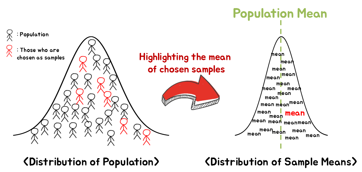
Figure 1. The process of extracting a sample from a population and calculating the statistics of the sample

On the left of Figure 1, the population is represented. For instance, the population could be the heights of several hundred people.

We can select a random sample from the left population and calculate the mean of these height values.

At this point, one might wonder if the mean of the sample we selected randomly (red in the right distribution) has a special meaning. When considering this, it should be remembered that these samples are not the sample mean values that have any special meaning. This is because the selection of samples was random.

Therefore, there will be countless cases related to the sample selection, and if we collect the mean values of those different cases, they will take the shape of the sample mean distribution on the right of Figure 1 ¹.

Looking closely at the shape of the sample mean distribution in Figure 1, it can be seen that it follows a normal distribution². Also, it is a well-known fact that the range of 2 * standard deviation from the mean value in a normal distribution occupies about 95% of the area³.

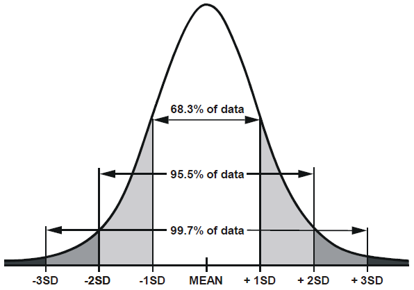
Figure 2. The area from the mean to ±2 standard deviations in a normal distribution is about 0.95.
Image source: Loony Labs

So how is the standard deviation calculated in the sample mean distribution?

As seen in The meaning of samples and standard error, the standard deviation of the sample mean is called “Standard Error of Mean (SEM),” and its value is

\[SEM = \frac{\sigma}{\sqrt{n}}\]

Here, $\sigma$ represents the standard deviation of the population, and $n$ represents the sample size (i.e., how many people were selected to calculate the average).

In other words, we can draw the following conclusion:

“The sample mean that I just extracted is within 95% confidence interval, which is within 2 times the standard error (SEM) range from the population mean.”

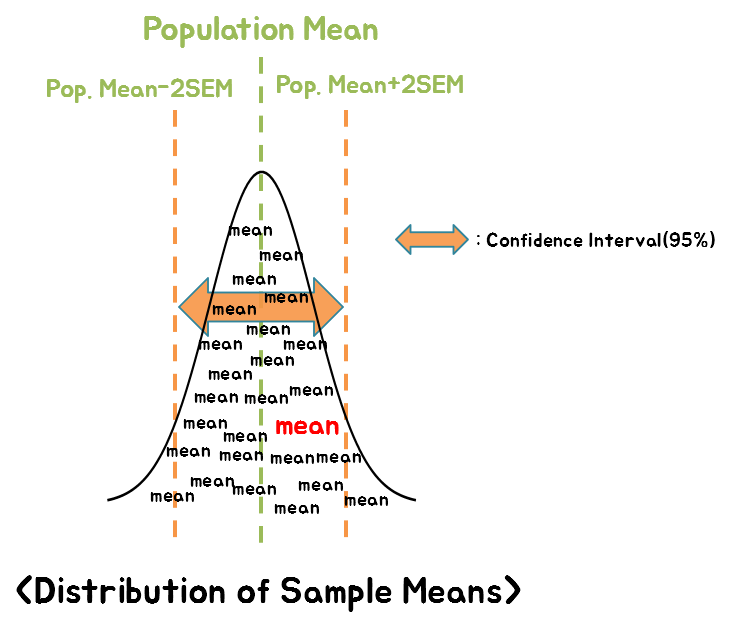
Figure 3. The sample mean is within the ±2SEM range from the population mean with a 95% probability.

However, there is a big problem here. We do not know the population mean.

If we knew the population mean, we wouldn’t have needed to extract samples and calculate the sample mean in this way.

So, let’s think about the relationship between the sample mean and the population mean from a slightly different perspective.

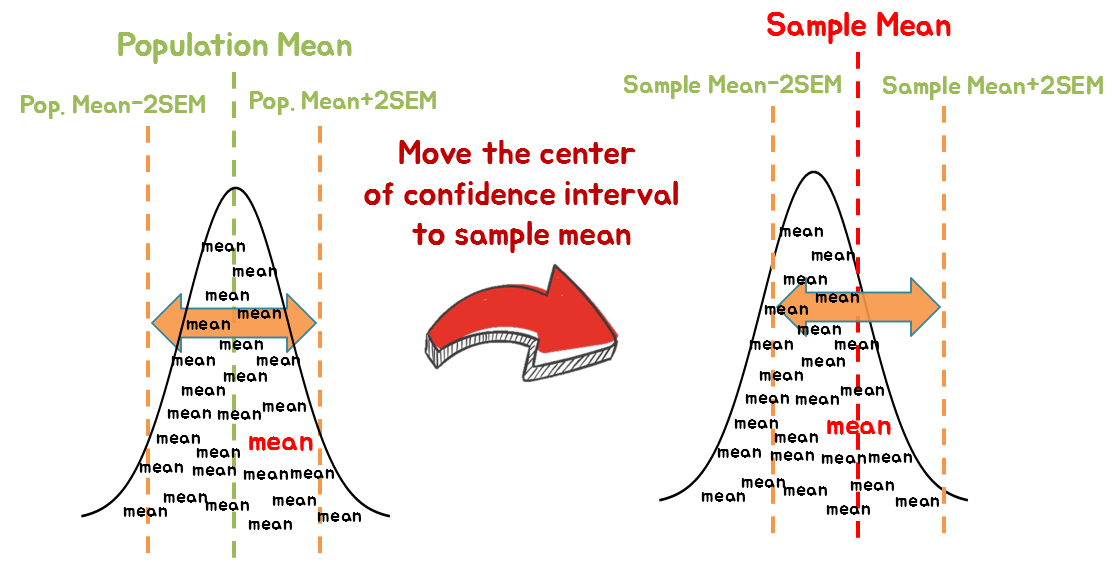
Figure 4. We can say that there is a 95% probability that the population mean is within ±2 standard errors from the sample mean.

As we can see in Figure 4, if we shift the interval that is 2SEM away from the population mean to be centered on the sample mean, we can know that the population mean is within ±2SEM from the sample mean with a 95% probability.

Thinking of the fact that there are countless combinations for sample extraction, we can also think that, if we repeat the sampling process about 100 times, 95 times, or so, the population mean would be within 2 times the standard error.

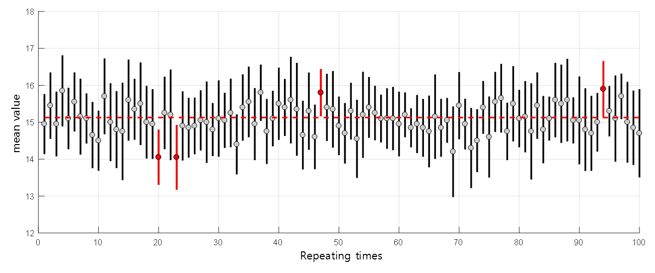
Figure 5. The fact that the population mean is within the 95% confidence interval of ±2SEM means that the population mean is contained within the range of ±2SEM about 95 times when repeating the sampling process 100 times.
The red horizontal dotted line represents the population mean, and the black vertical interval that overlaps with the horizontal line includes the population mean. The red vertical interval does not include the population mean.

What are margin of errors and confidence intervals?

Figure 6. A message seen every time there is an election. 'margin of error'
Source: BBC

In the previous post, we used the term ‘95% probability,’ but in some cases, the word probability is replaced by the term ‘margin of errors.’ In other words, we can say that the term ‘margin of error’ goes hand in hand with the term ‘probability.’

For example, let’s say we conducted a poll on the approval rates of candidates A and B in an opinion poll with a confidence level of 95% and a margin of error of ±3% (i.e., 2 x SEM = 3%), which is seen during every election. Assume that the survey results of 100 people show approval rates of 40% and 36% for candidates A and B, respectively. Based on the given information of 95% confidence level and ±3% margin of error, there is a 95% chance that the true proportion of A’s approval rate is between 37-43%, and the true proportion of B’s approval rate is between 33-39%.

Here, the two ranges, 37-43% and 33-39%, for candidates A and B, respectively, are the 95% confidence intervals for candidates A and B.

If you understood this much, you can also understand that there is a possibility that B’s true proportion is higher than A’s. This is because the true proportion of A’s approval rate could be 37%, and the true proportion of B’s approval rate could be 39%.

Confidence Interval for Comparing Two Groups (Using t-value)

Review of t-distribution

In the previous post on t-values and Student’s t-test, we learned about the t-distribution.

In this post, we will explain confidence intervals using the t-distribution. If you can understand confidence intervals using the t-distribution, you can understand estimating the population mean with small sample sizes or comparing two sample groups. To do this, let’s revisit the characteristics of the t-distribution.

First, what we can immediately notice from the t-distribution is that it is similar to the normal distribution. Why is that? It’s because both the normal distribution and t-distribution are distributions related to the mean. According to the Central Limit Theorem, as the sample size increases, the distribution of sample means approaches the normal distribution. The t-distribution can be thought of as the distribution of sample means when the sample size is not very large in this process (although the distribution of the population should still follow the normal distribution). If we directly compare the shapes of the normal distribution and t-distribution, they look like the following:

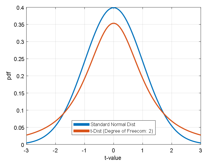
Figure 7. Comparison of the shapes of the standard normal distribution and t-distribution

As we can see in Figure 7, when comparing the shapes of the standard normal distribution and t-distribution, they look almost the same. The only difference is that the height of the peak at $t=0$ for the t-distribution is slightly lower, but the values at the ends (usually called the tails) look a bit higher.

Secondly, as we can see from the legend in the upper right corner of Figure 7, there is a concept called “degrees of freedom”. Degrees of freedom are a value directly related to the sample size and determine the shape of the t-distribution. As we can see in Figure 8, as the degree of freedom increases, the shape of the t-distribution becomes closer to the shape of the normal distribution.

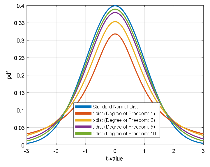
Figure 8. Comparison of the shapes of the standard normal distribution and t-distribution

Lastly, what we want to address about the t-distribution is the area under the curve. This is the most important part of this review of the t-distribution, so make sure you understand it before moving on. When calculating probabilities using the probability density function, we can use the area under the curve of the graph. For example, if we consider the t-distribution with 10 degrees of freedom and t values between 0 and 1, the area under the curve is represented by the red area in Figure 9, and it is equal to 0.3296.

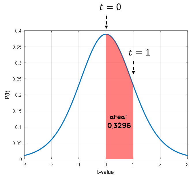
Figure 9. Comparison of the shapes of the standard normal distribution and t-distribution

At this time, what the area of 0.3296 means is that when the degree of freedom is 10, the probability that the t-value will be obtained between 0 and 1 is 0.3296.

(If you do not understand the meaning of the phrase “obtaining t-values”, it is recommended that you read t-value and Student’s t-test at least once.)

The major probability values (i.e., the width of the distribution) commonly used in statistical estimation are 0.95 and 0.99. Therefore, if we know the t-values that must be integrated from some t-value to another t-value around 0 in the t-distribution to obtain values of 0.95 or 0.99, estimation can be facilitated.

As shown in Figure 10, when the degree of freedom is 10, the t-values corresponding to the t-distribution area of 0.95 or 0.99 are ±2.228 and ±3.169, respectively.

A t-value table has been prepared for several degrees of freedom through such investigations.

As seen in the t-value table, “df” is written on the far left, followed by numbers from 1 to 1000. This is the degree of freedom. The t-distributions used in Figure 9 and Figure 10 both had a degree of freedom of 10. Therefore, to find the t-value we are looking for using the t-value table in Figure 11, we must look at the row corresponding to df=10.

Then, we need to find the column we are looking for. In the top row of Figure 5, we can see a value labeled t.975 and another labeled “two-tails 0.05.” This value is the t-value corresponding to a probability of 0.95 when excluding both tails.

By using the appropriate degree of freedom and the desired area, we can obtain t-values of 2.228 and 3.169.

In summary, we discussed the characteristics of the t-distribution, including its shape and degrees of freedom, and also mentioned that probabilities can be calculated by computing the area under the probability density function.

Finally, we talked about t-values that can obtain a specific area. In this post, we will write “$t_{0.95}$” for the t-value that can obtain an area of 0.95 by cutting the tails on both sides. We will also generalize it as “$t_A$,” which is the t-value that cuts off the tails on both sides and leaves an area of $A$.

Confidence Interval Setting in t-test

Earlier, we derived the definition of the confidence interval for the population mean of the sample mean by considering the concept of the population mean when thinking about the concept of the sample mean.

One of the other results we want to obtain through statistical analysis is the comparison between sample groups.

In particular, the most commonly used parametric statistical technique for comparing the means of two sample groups is the t-test, and we covered the content on the t-test in the meaning of t-value and Student’s t-test.

The point to pay attention to in constructing the concept of a confidence interval for the t-test is the hypothesis setting when performing the t-test.

The hypothesis when performing the t-test was as follows:

"The two sample groups came from one population."

Therefore, the obtained result is the t-value, and a larger t-value indicates a lower likelihood that the two sample groups came from the same population.

This is because the t-value is defined as the difference between the sample means in the numerator, as shown in Figure 12, so the farther the distance between the means, the larger the t-value.

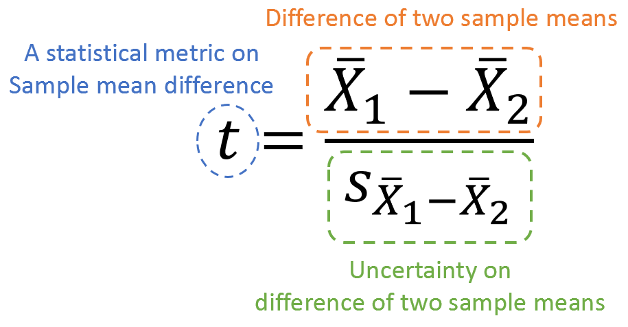
Figure 12. Formulaic definition of t-value and the meanings of each element

Now, in this session, let’s reverse the hypothesis of the t-value. In other words, let’s assume that the two samples were extracted from groups with different population means.

Reversing the existing assumptions about the t-test in this way is to adopt the method of obtaining the concept of a confidence interval by thinking about the population mean when determining the confidence interval for the sample mean. If this sounds a bit difficult, it might be helpful to first review the explanation in the figure below and then read this part again.

Then, let’s consider the process of comparing the sample means by extracting samples from different populations in earnest.

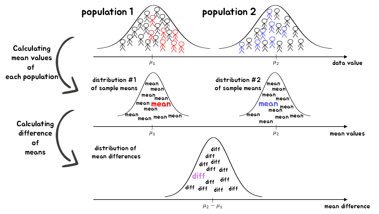
Figure 13. The process of comparing the means of two sample groups

그림 13에서는 서로 다른 두 모집단에서 표본을 추출한 뒤 각 표본 평균을 계산하였다. 그 뒤에 평균값의 차이에 관한 분포에 지금 뽑은 두 표본 평균의 차이를 표시하였다. 그림 13의 가장 아래에 표현된 그림을 따로 떼서 표현하면 그림 14와 같이 그릴 수 있다. 그런데 생각해보면 그림 14는 그림 3과 매우 유사하다. 즉, 우리의 두 표본의 차이는 모평균의 차이로부터 양 옆으로 어느 정도 크기의 확률로 들어온다는 것이라는 해석이 가능하다는 것을 말해준다.

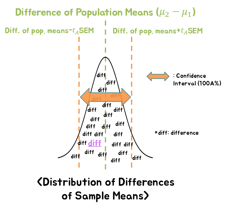
그림 14. 표본 평균의 차이는 모평균 차이로부터 ±$t_A$ SEM 범위 안에 100A% 확률로 포함되어 있다.

As seen in the t-distribution review section, the probability that a value is $t_A$ away from the center can be interpreted as $100A$, and as shown in Figure 12, the t-value is defined as the difference between the means divided by the standard error of the mean.

Therefore, we can know that the probability that the difference between our sample means falls between $\pm t_A\times SEM$ from the population mean is $100A$.

However, since we do not know the actual difference in population means, we apply the method we used for the sample mean to shift the confidence interval for the sample mean difference around the population mean.

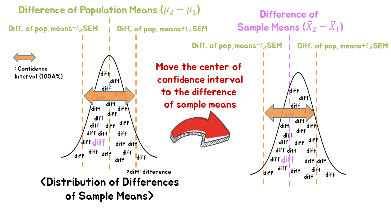
Figure 15. We can say that there is a 100A% probability that the population mean is included in the range of ±$t_A$SEM from the difference between sample means.

Then we can obtain the following conclusion:

The difference between the two population means exists within $\pm t_A SEM$ from the sample mean with a probability of 100A%.

For example, let’s say we want to compare two sample groups. Suppose we are curious about the difference in average height between adult Korean men and women. In this case, let’s randomly select 6 men and 6 women and measure their height.

\[\text{Men's sample group (6 people): }[170, 165, 168, 180, 175, 174]\] \[\text{Women's sample group (6 people): }[165, 162, 158, 170, 163, 154]\]

Calculating the sample mean values from this data, we have:

The sample mean for the men’s group is as follows.

\[\bar{X}_1= 172\]

The sample mean for the women’s group is as follows.

\[\bar{X}_2= 162\]

The standard deviation of the men’s sample is as follows.

\[s_1 = 5.40\]

The standard deviation of the women’s sample is as follows.

\[s_2 = 5.55\]

The standard deviation of two samples cannot be the same. However, the t-test is based on the assumption that the two samples are drawn from the same population. Therefore, we need to calculate a representative value for the two standard deviations, called the pooled standard deviation. The pooled standard deviation can be calculated as follows:

\[s = \sqrt{\frac{1}{2} (s_1^2 + s_2^2)} = 5.48\]

Using this, the standard error of the mean (SEM) can be calculated as follows:

\[s_{\bar{X}_1-\bar{X}_2} = \sqrt{\frac{s^2}{n_1}+\frac{s^2}{n_2}} = 3.16\]

The degrees of freedom for this t-test are 6+6-2 = 10, and the t-value corresponding to an area of 0.95 in both tails with 10 degrees of freedom is

\[t_{0.95} = 2.228\]

Therefore, the length of the 95% confidence interval is

\[t_{0.95} \times SEM = 2.228 * 3.16 = 7.04\]

Thus, the 95% confidence interval for the difference in mean height between men and women is

\[(\bar{X}_1 - \bar{X}_2)\pm t_{0.95}\times SEM = 10\pm 7.04\]

In other words, we can be 95% confident that the difference in mean height between men and women is between 2.96 and 17.04 cm.

In summary, if someone asks what the height difference is between Korean adult men and women, we can calculate the values by randomly selecting six people from each group and using the above formula to estimate that men are 2.96 cm to 17.04 cm taller than women with 95% confidence.

p-value may not be sufficient alone.

Despite the existence of a convenient and excellent tool called p-value, why do we need a new concept called confidence intervals?

The statistical result processing techniques used in the statistical techniques we have studied so far, such as the t-test, ANOVA, etc., are primarily used to indicate whether to reject the null hypothesis.

Rejecting the null hypothesis means that the null hypothesis and the current result cannot be reconciled. We express the degree of compatibility that can be reconciled using the p-value.

In other words, p-value is a probability value that tells us how well the null hypothesis and the current result are compatible.

Therefore, obtaining a low p-value (usually below 0.05) means that the null hypothesis and the current experimental results do not match, and the null hypothesis is rejected.

However, as we saw in the meaning of p-value, the p-value is a compressed number that contains a lot of information. The information that p-value contains can be broadly divided into two: the effect size and the sample size. However, p-value expresses these two pieces of information in a single number. Therefore, even if we obtained a very small p-value as a result of our experiment, we cannot tell whether the cause of the fact that we can reject the null hypothesis is because the effect size is sufficiently large, or because the sample size is large, resulting in the obtained results, using only the p-value value.

Figure 16 below shows the desirable case where the value of p-value becomes small as the effect size increases.

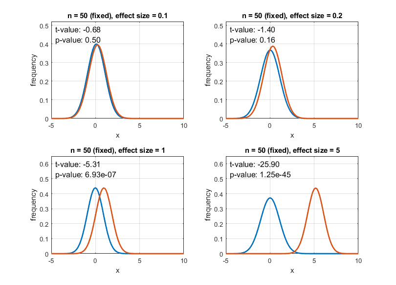
Figure 16. Distribution of two groups according to various effect sizes and p-values

On the other hand, Figure 17 below shows the case where the value of p-value becomes small enough to reject the null hypothesis even though the effect size is small due to the large sample size. This case may not be desirable.

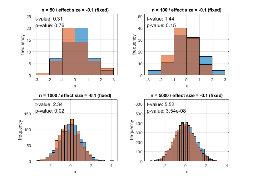
Figure 17. Distribution of two groups according to various sample sizes and p-values

Therefore, when interpreting research results statistically, it is more desirable to not only provide ‘reject/accept’ decisions using only p-values but also to allow the interpretation of the treatment effect size.

To understand this content more specifically, let’s try to solve a problem.

Let’s imagine that a new medication has been developed that lowers blood pressure. To demonstrate its efficacy, let’s say that 100 individuals were selected for both the medication and placebo groups and appropriate medication was prescribed to each group to obtain blood pressure values.

For instance, let’s say that the mean diastolic blood pressure of the medication group was 81 mmHg with a standard deviation of 11 mmHg. Also, let’s say that the mean diastolic blood pressure of the placebo group was 85 mmHg with a standard deviation of 9 mmHg.

If we were to draw a histogram, we could consider the following data:

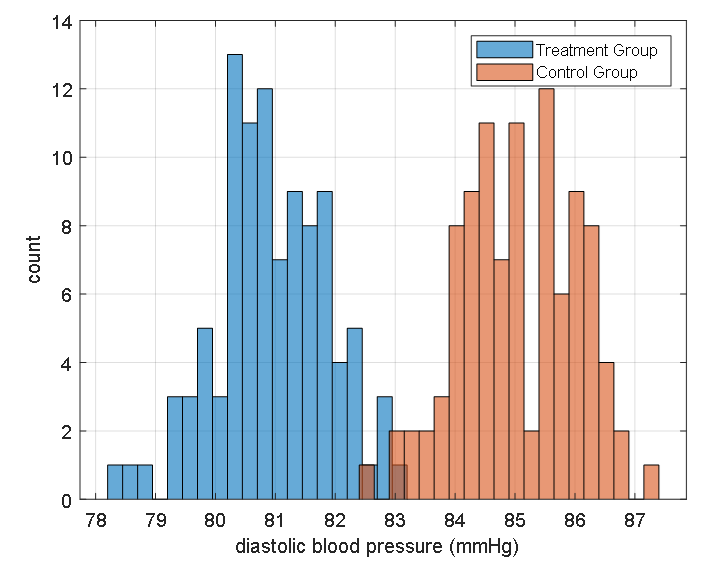
Figure 18. Expected distribution of the blood pressure medication's treatment group and control group.

Can we say that the two sample groups (medication and placebo) match the null hypothesis that there is no difference? To answer this question, a t-test must be performed.

To calculate the t-value, we first calculate the pooled variance as:

\[s^2 = \frac{1}{2}(11^2+9^2) = 10^2\text{ mmHg}\]

Thus,

\[t=\frac{\bar{X}_{dr} - \bar{X}_{pla}}{s_{\bar{X}_{dr} - \bar{X}_{pla}}}=\frac{81-85}{\sqrt{(10^2/100)+(10^2/100)}}=-2.83\]

We can see that the t-value is -2.83.

As this t-value is smaller than the t-value for p-value = 0.01, which is $t=-2.61$, we can confirm statistically that the medication significantly lowers blood pressure with a p-value less than 0.01.

However, can we say that this result is clinically significant, as well as statistically significant?

The t-value for a two-sided tail, excluding the tail parts in both directions that correspond to a probability of 0.95 and degrees of freedom of 198 (=100+100-2) is:

\[t_{0.95} = 1.972\]

In addition, the standard error is:

\[s_{\bar{X}_{dr} - \bar{X}_{pla}} = \sqrt{(10^2/100)+(10^2/100)} = 1.41\]

Therefore, the 95% confidence interval for the difference in population means is

\[-4-1.972(1.41)<\mu_{dr}-\mu_{pla}<-4+1.972(1.41)\] \[-6.8\text{ mmHg}<\mu_{dr}-\mu_{pla}<-1.2\text{ mmHg}\]

From this result, it can be said that the extent to which the new drug lowers blood pressure is about -1.2 ~ -6.8 mmHg, but considering that the standard deviation of each group is 9 or 11, the drug is considered to have a very weak effect in lowering blood pressure. In other words, statistically significant differences were found in the data, but clinically the drug may not have a significant effect when actually used.

What can be learned here is that using confidence intervals that show the magnitude of the treatment effect in addition to p-values can provide more information for analyzing experimental results, making it easier to analyze the results.