이 문서의 한국어 버전은 아래의 위치에서 찾을 수 있습니다. (You can find a Korean version of this article as below.)
What the CT convolution means: A continuous function can be represented by breaking it down into smaller pieces.
Prerequisites
To better understand this post, it is recommended that you have knowledge of the following topics:
1. Meaning of Discrete Signal Convolution [Review]
In this session, we will consider convolution in the continuous-time domain. In mathematics, we typically learn about continuous-time signals (i.e., real-valued functions) first and then learn about discrete-time signals when we come to college. However, in many cases, it is helpful to first think about concepts in the discrete-time domain and then extend them to the perspective of continuous-time signals to aid understanding.
In discrete-time, convolution can be understood as decomposing an arbitrary function $x[n]$ using the delta function $\delta [n]$. In mathematical notation, this can be written as below.
\[x[n]=\cdots + x[-2]\delta[n+2]+x[-1]\delta[n+1]+x[0]\delta[n]+x[1]\delta[n-1]+x[2]\delta[n-2]+\cdots \notag\] \[= \sum_{k=-\infty}^{\infty}x[k]\delta[n-k] = \sum_{k=-\infty}^{\infty}x[n-k]\delta[k]\]So, if we take a closer look at equation (1), we can see that the function $x[n]$ can be represented as “function value $\times \delta[n]$”. Then, can’t we decompose an arbitrary continuous-time signal $x(t)$ using function values and delta function as well?
Discrete signals can be seen as samples of continuous signals in some cases. If we want to understand the concept of convolution for continuous signals starting from the concept of convolution for discrete signals, the connecting link can be found in sampling. Therefore, let’s introduce a simple method of sampling for continuous signals.
2. Sampling Method for Continuous-Time Signals: Sample and Hold
One of the simplest methods for sampling a continuous-time signal is sample and hold. Sample and hold involves measuring the analog signal and then maintaining its value for one sampling period. In this post, we will briefly introduce the concept of 0th order sample and hold.
In the figure below, the gray signal represents the original signal, and the red line represents the signal sampled using 0th order sample and hold.

Figure 1. 0th order sample and hold
0th order sample and hold is very simple. It involves measuring (or acquiring) the value of the signal at a specific time and maintaining that value until the next sampling period. In this post, we will use a similar approach with the rect function to sample continuous-time signals. The difference from the Wikipedia figure is that in this post, as indicated by the red arrow at the top of the post, the sampled value of the continuous-time signal is located at the center of the rectangular pulse, rather than the left top corner of the rectangular pulse.
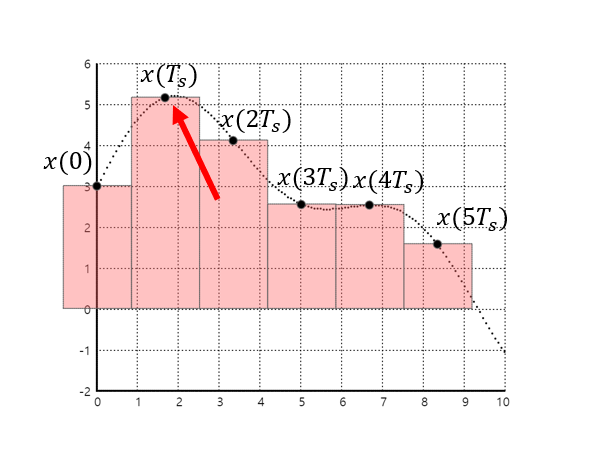
Figure 2. Sampling continuous signal using rectangular pulses.
3. Mathematical Representation of Sampled Signal
In the figure above, the graph on the left-hand side represents the signal obtained by sampling the continuous-time signal at intervals of $T_s$. The graphs on the right-hand side indicate that the signal on the left-hand side can also be represented as the sum of shifted rectangular pulses, each with an amplitude equal to the sample value.
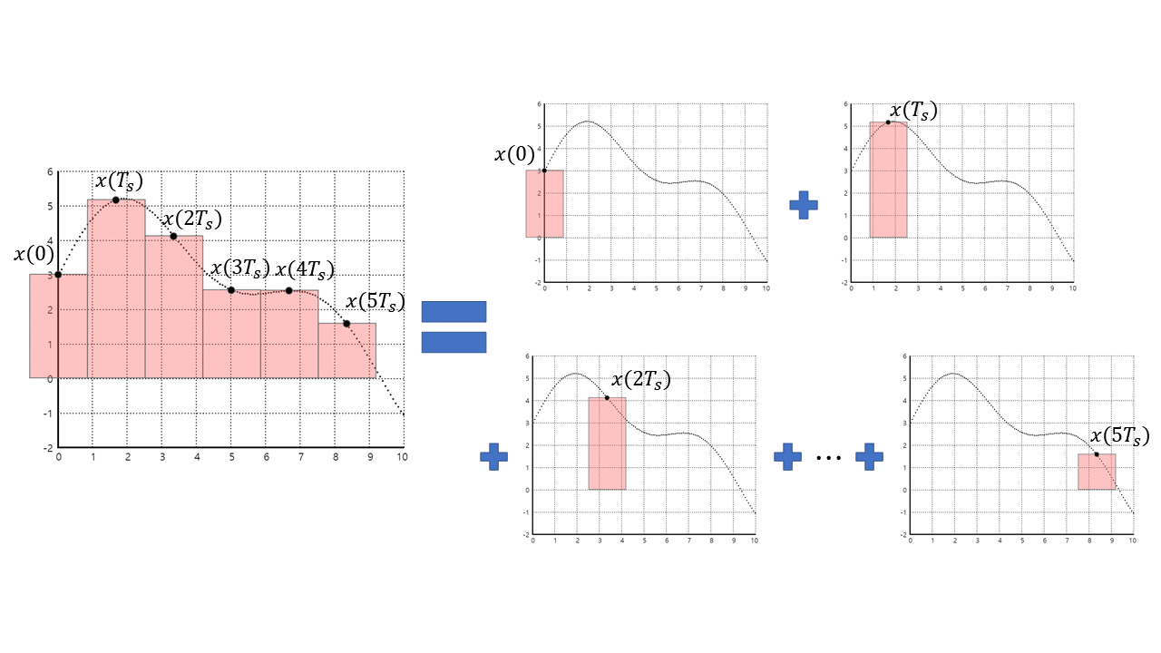
Figure 3. Sampled signal can also be represented as the sum of shifted rectangular pulses, each with an amplitude equal to the sample value.
Each individual red square on the right-hand side of the figure can be mathematically represented as a rectangular pulse.
| DEFINITION 1. Rectangular pulse |
|---|
| A rectangular pulse $\Pi(t)$ can be defined as follows. |

Figure 4. The shape of a rectangular pulse
When a rectangular pulse is shifted by “a” and scaled by “b”, the resulting waveform is as follows:
\[\Pi\left(\frac{t-a}{b}\right)\]
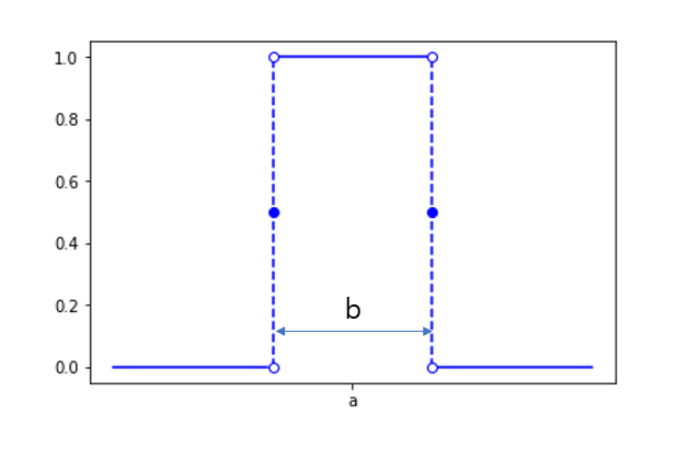
Figure 5. Rectangular pulse shifted and scaled
Using the definition of a rectangular pulse, the sampled signal of $x(t)$ from Figure 3 can be expressed as follows:
\[x(t) \rightarrow (sampling) \rightarrow \sum_{k=-\infty}^{\infty}{x(k T_s) \frac{1}{T_s} \Pi\left(\frac{t-kT_s}{T_s}\right)}\]The inclusion of $1/T_s$ in the above equation is to normalize the results and prevent changes in the results depending on the length of the sampling period $T_s”.
4. Continuous Signal Convolution
If the sampling period in a sampled signal of a continuous signal is made very short, the original continuous signal can be perfectly restored.
Therefore, the following equation can be written by taking the limit of $T_s$ approaching zero:
\[\lim_{T_s\rightarrow 0}\left\{\sum_{k=-\infty}^{\infty}{x(k T_s) \frac{1}{T_s} \Pi\left(\frac{t-kT_s}{T_s}\right)}\right\}\]The process represented in the above equation is shown in the animation at the top of this post, where the slider is moved to the right.
In this equation, it can be understood that the part $x(kT_s)$ represents the function values as $T_s$ approaches very small values, and the part $\frac{1}{T_s} \Pi(\frac{t-kT_s}{T_s})$ can be understood by defining it as a delta function.
| DEFINITION 2. Continuous Time Delta Function (Dirac Delta function) |
|---|
| One of ways to represent Dirac delta function is as below. |
Therefore, equation (5) can be expressed as follows by the definition of definite integral and delta function:
\[\lim_{T_s\rightarrow 0}\left\{\sum_{k=-\infty}^{\infty}{x(k T_s) \frac{1}{T_s} \Pi\left(\frac{t-kT_s}{T_s}\right)}\right\} = \int_{-\infty}^{\infty}{x(k) \delta(t-k)dk}\]In signal theory, $\tau$ is often used instead of $k$.
5. Impulse Response in Continuous Time Domain
Similar to the case of DT signals, using the properties of Linear Time Invariant (LTI) systems,
the input-output relationship can be expressed as a linear operator $O$:
\[y(t) = O_n\{x(t)\}\]Then, according to the definition of continuous convolution shown earlier,
\[= O_n\left\lbrace\int_{-\infty}^{\infty}{x(k) \delta(t-k)dk}\right\rbrace\]By the properties of LTI systems,
\[=\int_{-\infty}^{\infty}{x(k) O_n\{\delta(t-k)\}dk}\]And by the definition of impulse response,
\[=\int_{-\infty}^{\infty}{x(k) h(t-k)}\]Where $h(t)$ is the impulse response. In general, using $\tau$ instead of $k$, the relationship between input, output, and impulse response can be expressed as1.:
\[y(t) = \int_{-\infty}^{\infty}{x(\tau)h(t-\tau) d\tau}\]-
I recommend referring to a more detailed post on discrete time convolution, specifically regarding the derivation of the relationship between input, output, and impulse response using LTI (Linear Time-Invariant) systems: Discrete Convolution ↩