The method of matrix multiplication commonly used

When I was in high school, I learned about matrices. The multiplication method for matrices that I first learned was so unique that even now, if you’re not familiar with it, you might think “Why is matrix multiplication done like this?”.

Matrix multiplication is generally thought of as follows:

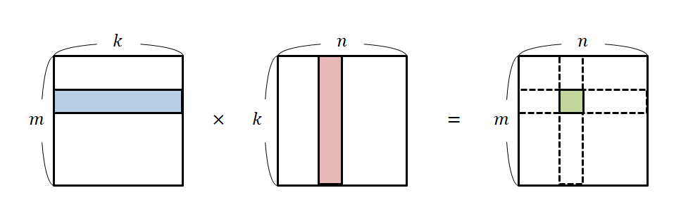
Figure 2. The general method of matrix multiplication

To express this formula more accurately using notation, we have:

\[\begin{bmatrix} 1 & 2 \\ 3 & 4 \end{bmatrix}\begin{bmatrix}a & b \\ c & d\end{bmatrix} = \begin{bmatrix} 1 \cdot a +2\cdot c && 1\cdot b + 2\cdot d \\ 3\cdot a + 4\cdot c && 3\cdot b + 4 \cdot d\end{bmatrix}\]

If you examine this more closely, you can see that it involves taking one row from the matrix on the left and one column from the matrix on the right and then performing a calculation.

The reason matrix multiplication is defined in this way is that matrices can be seen as a type of function.

To be more precise, let’s think of a matrix as a function $f, g: \Bbb{R}^2\rightarrow \Bbb{R}^2$ that takes a 2-dimensional vector as input and outputs a 2-dimensional vector.

In other words, for the vector $[x,y]^T$ and the matrices $f$ and $g$ below (where we emphasize the meaning of mapping by writing them as $f$ and $g$):

\[f: \begin{bmatrix} a & b \\ c & d \end{bmatrix}\] \[g: \begin{bmatrix} p & q \\ r & s \end{bmatrix}\]

Each mapping is as follows:

\[f\left(\begin{bmatrix} x \\ y\end{bmatrix}\right)=\begin{bmatrix}ax+by \\ cx+dy\end{bmatrix}\] \[g\left(\begin{bmatrix} x \\ y\end{bmatrix}\right)=\begin{bmatrix}px+qy \\ rx+sy\end{bmatrix}\]

If we consider the composition of the two mappings, $f\bullet g$, we have:

\[f\bullet g\left(\begin{bmatrix} x \\ y\end{bmatrix}\right) =\begin{bmatrix}a(px+qy)+b(rx+sy) \\ c(px+qy)+d(rx+sy)\end{bmatrix}\] \[=\begin{bmatrix}(ap+br)x + (aq+bs)y \\ (cp+dr)x + (cq+ds)y\end{bmatrix}\]

Therefore, the composite mapping $f\bullet g$ is defined as follows.

\[f\bullet g=\begin{bmatrix} ap+br & aq+bs \\ cp+dr & cq+ds\end{bmatrix}\]

This composite mapping is defined as a matrix product, and is represented by writing the two matrices side by side without using any special operation symbols¹.

Also, if we think of the imported rows or columns as vectors, we can see that each element of the calculated matrix represents the inner product of vectors.

In other words, the value of the element in the first row and first column of equation (1) represents the inner product of the row vector of the left matrix and the column vector of the right matrix before calculation.

\[\begin{bmatrix}1 & 2\end{bmatrix}\begin{bmatrix}a\\c\end{bmatrix} = 1\cdot a + 2\cdot c\]

Thus, we can see that the commonly used perspective of matrix multiplication involves computing the inner product of row vectors and column vectors.

It is important to note that the operation is between a row vector and a column vector, not between two row vectors or two column vectors. For further information on this point, I recommend referring to the next post, Meaning of Row Vectors and Inner Products.

As an application of this perspective, there is the concept of covariance matrix, which means how similar various features are to each other (i.e., using inner product).

Linear Combination of Column Vectors

Another way to understand matrix multiplication is to think of it in terms of linear combinations of column vectors.

Let’s think about the product of a matrix and a vector. In other words, let’s check the result by taking only one column of the matrix that is multiplied on the right-hand side in equation (1).

\[\begin{bmatrix} 1 & 2 \\ 3 & 4 \end{bmatrix}\begin{bmatrix}a \\ c \end{bmatrix} = \begin{bmatrix} 1 \cdot a +2\cdot c \\ 3\cdot a + 4\cdot c \end{bmatrix}\]

Looking at this result, we can also think of it in the following way:

\[\begin{bmatrix} 1 & 2 \\ 3 & 4 \end{bmatrix}\begin{bmatrix}a \\ c \end{bmatrix} = a\cdot\begin{bmatrix} 1\\ 3 \end{bmatrix} + c\cdot\begin{bmatrix} 2\\ 4\end{bmatrix}\]

In other words, we can say that the product of a matrix and a vector is another way of representing the linear combination of the two column vectors that make up the matrix.

Interpretation based on Column Space

As explained in the section on Linear Combination of Vectors, the linear combination of vectors refers to the generation of a vector space. Therefore, the formula of multiplying matrices and vectors asks us to explore the vector space (i.e., the column space) that can be created using the given column vectors, which is very important.

From this perspective, let’s think about the meaning of the following formula.

\[A\vec{x} = \vec{b}\]

For example, consider the following problem:

\[\begin{bmatrix}1 & 2 \\ 3 & 4\end{bmatrix}\begin{bmatrix}x\\y\end{bmatrix}=\begin{bmatrix}3\\5\end{bmatrix}\]

The solution to this problem can be easily found by solving the system of equations, as follows:

\[\begin{cases}x+2y = 3 \\3x+4y = 5\end{cases}\] \[\Rightarrow x=-1, \text{ }y=2\]

However, let’s think about this equation in a different way:

\[x\begin{bmatrix}1\\3\end{bmatrix}+y\begin{bmatrix}2\\4\end{bmatrix}=\begin{bmatrix}3\\5\end{bmatrix}\]

I want to interpret this equation as follows:

"Is the vector $\begin{bmatrix}3\\5\end{bmatrix}$ located within the vector space generated by the two vectors $\begin{bmatrix}1\\3\end{bmatrix}$ and $\begin{bmatrix}2\\4\end{bmatrix}$? If so, how can we combine $\begin{bmatrix}1\\3\end{bmatrix}$ and $\begin{bmatrix}2\\4\end{bmatrix}$ to obtain $\begin{bmatrix}3\\5\end{bmatrix}$?"

Applications of linear algebra using this perspective include solving linear equations and linear regression.

Interpretation Based on Linear Transformations

In addition, another interpretation that the product of a matrix and a vector is a linear transformation of the vector through the transformation of the basis vector, which is the perspective provided by the interpretation that the product of a matrix and a vector is a linear combination of column vectors.

For example, if we use the matrix

\[A=\begin{bmatrix} 2 & -3 \\ 1 & 1 \end{bmatrix}\]

to transform the vector

\[\vec x=\begin{bmatrix} 1 \\ 1 \end{bmatrix}\]

we can see that

\[A\vec x =\begin{bmatrix} 2 & -3 \\ 1 & 1 \end{bmatrix} \begin{bmatrix} 1 \\ 1 \end{bmatrix}=\begin{bmatrix} -1 \\ 2 \end{bmatrix}\]

As shown in the video below, this value can be expressed as a combination of the new two basis vectors, each multiplied by 1.

Since this content has been covered in detail in the post Matrix as a Linear Transformation, it may be helpful to refer to that post.

Applications of linear algebra using this perspective include eigenvalues and eigenvectors, principal component analysis (PCA), and singular value decomposition (SVD).