Prerequisites
We recommend having a good understanding of the following topics before proceeding:
- Meaning of the Central Limit Theorem
- Recommended JS Applet: Seeing Theory
- Maximum Likelihood Estimation (MLE)
- Recommended YouTube video: StatQuest
- Recommended JS Applet: Seeing Theory
- Gradient Descent
ICA Model and Objective
According to Wikipedia, Independent Component Analysis (ICA) is a computational method for separating multivariate signals into statistically independent subcomponents.
Although it may seem complicated, let’s understand what ICA can do by looking at the example below.
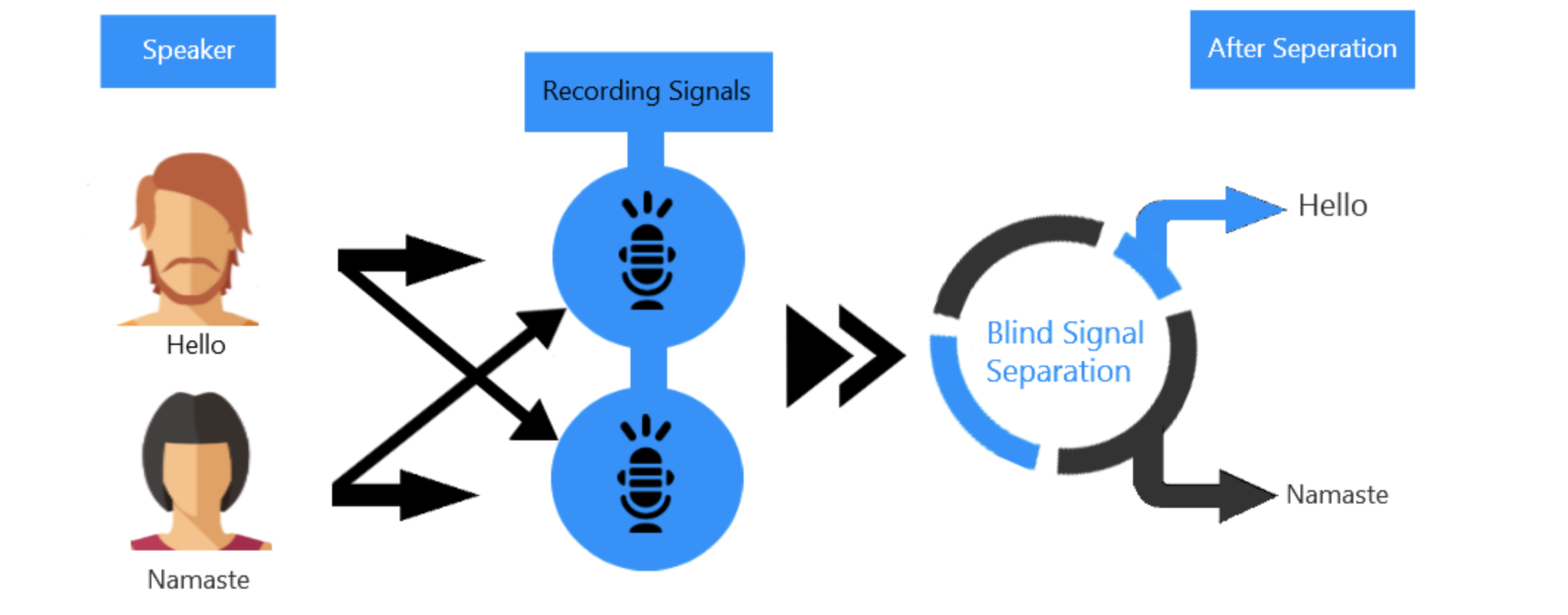
Figure 1. Block diagram illustrating what ICA can do.
It shows the process of separating two mixed audio sources.
(Labeled as Blind Source Separation, which is what ICA does)
Source: gowrishankar.info blog
Let’s consider a scenario where two people are speaking simultaneously in a room, and two microphones are recording the audio signals.
Let’s denote the recorded signals from the two microphones as $x_1(t)$ and $x_2(t)$, and the original speech signals from the two speakers as $s_1(t)$ and $s_2(t)$, respectively.
The relationship between these signals can be expressed as a set of linear equations:
\[x_1(t) = a_{11}s_1(t)+a_{12}s_2(t)\] \[x_2(t) = a_{21}s_1(t)+a_{22}s_2(t)\]Here, $a_{ij}$ with $i,j = 1, 2$ are variables related to the distances between the microphones and the speakers.
What we want to achieve is the separation of the original sources from the recorded audio signals, i.e., the recovery of $s_1(t)$ and $s_2(t)$.
The equations (1) and (2) can be represented as matrices as follows.
\[x = As\]Let’s call $A$ the mixing matrix.
Here, $x \in \mathbb{R}^n$, $A \in \mathbb{R}^{n \times n}$, and $s \in \mathbb{R}^n$.
If we know $A$, we can easily find the source $s$ by multiplying both sides with $A^{-1}$ on the left.
In other words, we can find the source using the following equation.
\[s = A^{-1}x = Wx\]Our goal is to find the unmixing matrix $W = A^{-1}$. However, how can we find the matrix $W$ without knowing the matrix $A”?
Central Limit Theorem and Independent Component Analysis
Understanding the Central Limit Theorem (CLT) is important to grasp the concept of Independent Component Analysis (ICA) because ICA is essentially the opposite of CLT.
In brief review, CLT states that the distribution of a linear combination of independent random variables tends to follow a Gaussian distribution.
Importantly, the more independent variables involved in the linear combination, the closer the distribution becomes to a Gaussian distribution.
The relationship between CLT and ICA can be depicted in the following figure.
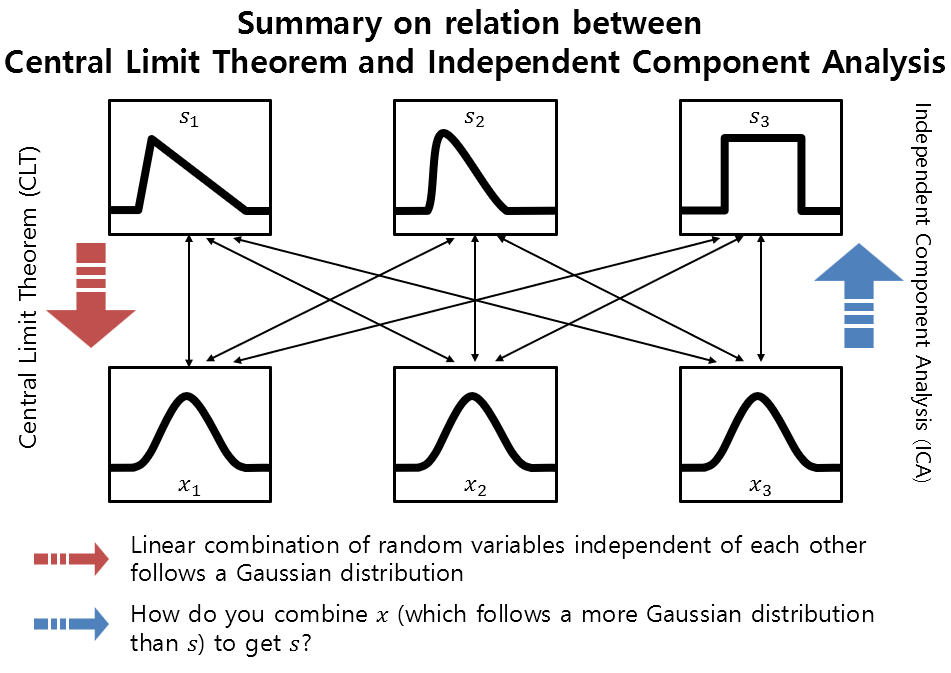
Figure 2. Overview of the relationship between Central Limit Theorem and Independent Component Analysis
In other words, if we think of ICA as the opposite process of CLT, ICA is the process of finding the original independent random variables, or sources, $s$, by multiplying the appropriate matrix $W = A^{-1}$ to the linear combination of independent random variables, or observed data, $x$, obtained from $s$.
In other words, in Independent Component Analysis (ICA), the goal can be seen as finding a matrix $W=A^{-1}$ that maximizes the satisfaction of the assumption that the sources are independent of each other.
Densities and linear transformation
As a final concept to understand the algorithm for Independent Component Analysis, let’s consider the relationship between the probability densities of variables before and after applying a linear transformation.
Since the total sum of the areas under the probability density functions should be 1, if we apply a linear transformation to a random variable using a matrix, we need to adjust the density function using the determinant of the matrix.
For example, let’s consider a random variable $s$ such that $s\sim Uniform[0,1]$, which means the density function of $s$ can be written as $p_s(s) = 1\lbrace s\leq 0 \leq 1\rbrace$.
Here, $1\lbrace condition\rbrace$ is a function that outputs 1 when the condition is satisfied, and 0 otherwise.
Now, let’s assume $A = 2$, and $x = As$, and $s = A^{-1}x = Wx$. Then, the correct expression for the density function of $x$ is not $’p_x(x) = p_s(Wx)’$, but rather $p_x(x) = p_s(Wx)\cdot |W|$, where $|W|$ denotes the determinant of the matrix $W$.
The following figure can help to understand this concept more easily.
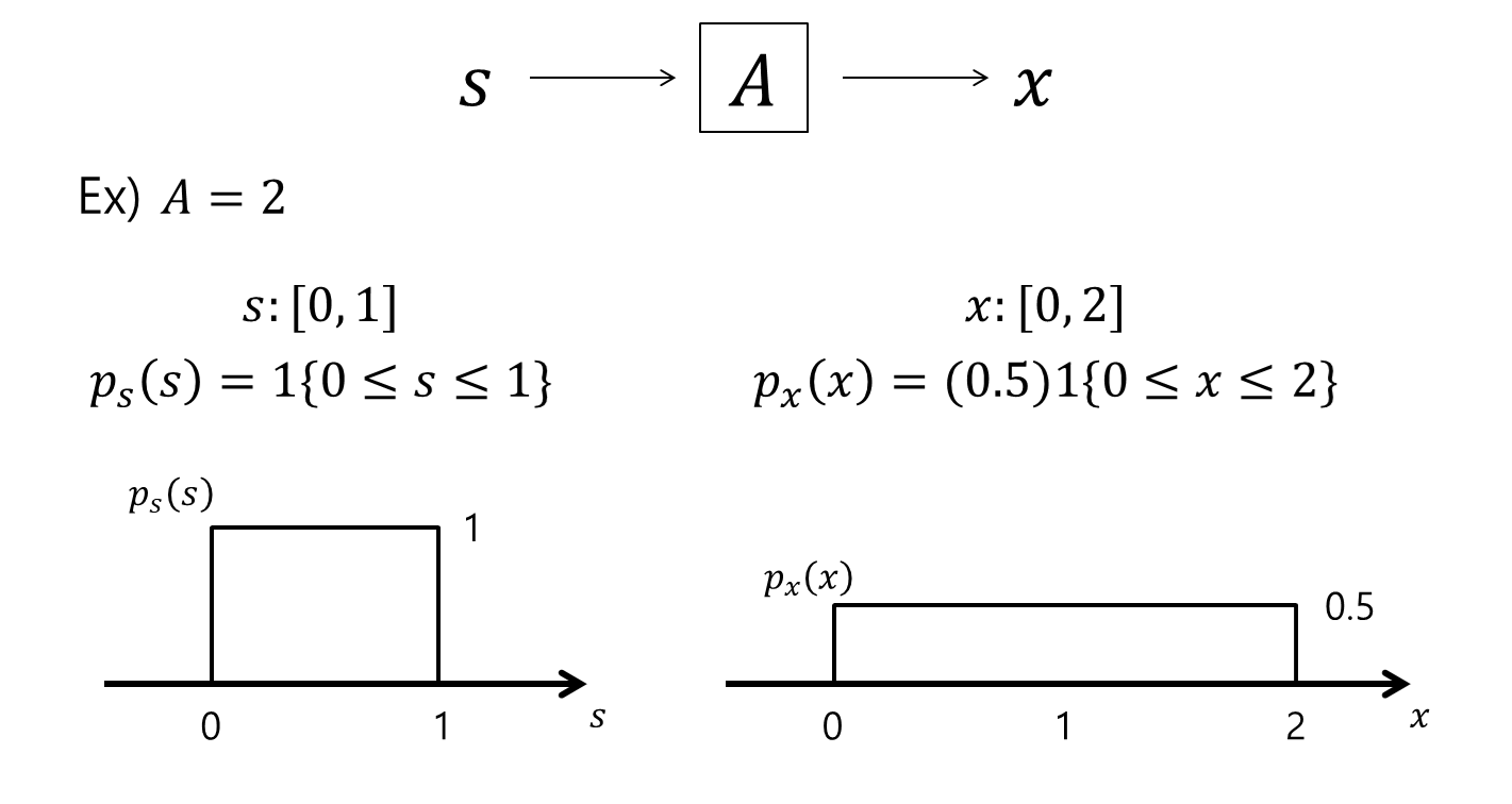
Figure 3. Example of probability density functions of random variables before and after applying linear transformation.
Therefore, considering that $x=As$ and $s=A^{-1}x=Wx$, we can express the probability density function of the random variable after linear transformation as follows:
In other words, we can calculate $p_x(x)$ in the following way:
\[p_x(x) = p_s(A^{-1}x))\cdot|A^{-1}|\notag\] \[= p_s(s)\cdot|A^{-1}|=p_s(Wx)\cdot|W|\]ICA algorithm
Bell-Sejnowski algorithm
If we denote the density function of each source $s_i$ as $p_s$, then the joint distribution composed of all sources can be written as follows:
\[p(s) = \prod_{i=1}^{n}p_s(s_i)\]As we saw in the previous section, given the relationship $x = As = W^{-1}s$, we can obtain the density function $p(x)$ as follows:
\[p(x) = \prod_{i=1}^{n}p_s(w_i^Tx)\cdot|W|\]We calculate $p(x)$ because the actual data we observe is not $s$ but $x$.
Now, let’s compute the log-likelihood of the density function $p(x)$ for the training samples we acquire, denoted as $\lbrace x^{(i)}; i = 1, 2, \cdots, m \rbrace$.
We calculate the likelihood to see which parameters among many can better explain the information we have obtained so far. In general, we compute the log-likelihood instead of the likelihood for convenience.
The log-likelihood for $m$ training data and $n$ sources can be computed as follows:
\[l(W) = \sum_{i=1}^{m}\left(\sum_{j=1}^{n}\log p_s(w_j^Tx^{(i)})+log|W|\right)\]Here, $w_j^T$ denotes the $j$-th row of the matrix $W$.
\[W = \begin{bmatrix}{ }- { } w_1^T { }- { } \\{ }- { } w_2^T { }- { } \\\vdots \\{ }- { } w_n^T { }- { } \\\end{bmatrix}\]Also, we can determine the specific probability density function for $p_s$.
It is generally known that there is no problem using the sigmoid function $g(s) = 1/(1+e^{-s})$ as the CDF of $p_s$ in the algorithm. (If prior knowledge about the density of the source is available, use that density function instead.)
Therefore, the pdf $p_s$ is $g’(s)$, and we can rewrite $l(W)$ as follows:
\[l(W) = \sum_{i=m}^{m}\left(\sum_{j=1}^{n}\log g'(w_j^Tx^{(i)})+log{|}W{|}\right)\]Now, let’s use the fact that $\nabla_W|W|=|W| (W^{-1})^T$ to take the partial derivative of $l(W)$ with respect to $W$.
At this point, for the convenience of expression, let’s replace $w_j^Tx^{(i)}$ with $s_j$ in order to simplify the formula.
\[\frac{\partial l}{\partial W} = \sum_{i=1}^{m}\left(\sum_{j=1}^{n}\frac{1}{g'(s_j)}\cdot g''(s_j)\cdot x^{(i)^T} + \frac{1}{|W|}|W|(W^{-1})^T\right)\] \[= \sum_{i=1}^{m}\left(\sum_{j=1}^{n}\frac{1}{g(s_j)(1-g(s_j))}\cdot g(s_j)(1-g(s_j))(1-2g(s_j))\cdot x^{(i)^T} + (W^{-1})^T\right)\] \[= \sum_{i=1}^{m}\left(\sum_{j=1}^{n}(1-2g(s_j))\cdot x^{(i)^T} + (W^{-1})^T\right)\]Using the Gradient Ascent method, $W$ can be updated as follows:
\[W := W + \alpha \frac{\partial l}{\partial W}\]Therefore, for each $j = 1, 2, \cdots, n$,
\[W := W + \alpha\left(\begin{bmatrix}1 - 2g(w_1^Tx^{(i)}) \\1 - 2g(w_2^Tx^{(i)}) \\\vdots \\1 - 2g(w_n^Tx^{(i)})\end{bmatrix} x^{(i)^T} + (W^T)^{-1}\right)\]Here, $\alpha$ is the learning rate.
After convergence of the above algorithm, the obtained $W$ can be used to obtain the original sources, $s$.
Natural Gradient Algorithm
The Bell-Sejnowski algorithm calculated earlier has a drawback in that it requires the calculation of the inverse term $(W^T)^{-1}$, which slows down the computation speed for updating $W$.
To address this issue, the natural gradient algorithm was developed, and its derivation process is not that difficult.
Multiplying $W^TW$ on the right-hand side of the term inside the parentheses in the formula (15) gives:
\[\left(\begin{bmatrix}1 - 2g(w_1^Tx^{(i)}) \\1 - 2g(w_2^Tx^{(i)}) \\\vdots \\1 - 2g(w_n^Tx^{(i)})\end{bmatrix} x^{(i)^T} + (W^T)^{-1}\right)W^TW\] \[=\left(\begin{bmatrix}1 - 2g(w_1^Tx^{(i)}) \\1 - 2g(w_2^Tx^{(i)}) \\\vdots \\1 - 2g(w_n^Tx^{(i)})\end{bmatrix} x^{(i)^T}W^TW + (W^T)^{-1}W^TW\right)\] \[=\left(\begin{bmatrix}1 - 2g(w_1^Tx^{(i)}) \\1 - 2g(w_2^Tx^{(i)}) \\\vdots \\1 - 2g(w_n^Tx^{(i)})\end{bmatrix} x^{(i)^T}W^T + I\right)W\]Therefore, by using the value obtained from equation (18) to update the weight, we can perform gradient ascent calculation a little faster without performing the inverse calculation.
\[W := W + \alpha \frac{\partial l}{\partial W}W^TW\]In other words, we can update $W$ through the following process:
\[W := W + \alpha\left(\begin{bmatrix}1 - 2g(w_1^Tx^{(i)}) \\1 - 2g(w_2^Tx^{(i)}) \\\vdots \\1 - 2g(w_n^Tx^{(i)})\end{bmatrix} x^{{(i)^T}}W^T + I\right)W\]Difference between PCA and ICA
※ If you are not familiar with PCA, click here.
Both PCA and ICA play a similar role in finding a set of basis vectors that represent the given data.
PCA finds a set of orthogonal basis vectors in the feature space.
In particular, PCA has the characteristic of selecting the basis vectors sequentially, which can yield the maximum variance when the data is projected onto them.
On the other hand, the basis vectors obtained through ICA may not be orthogonal to each other.
ICA has the characteristic of selecting basis vectors that make the projections of the data as independent (non-Gaussian) as possible.
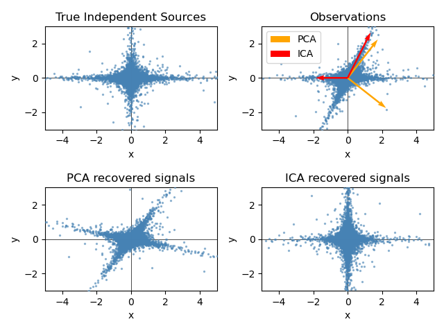
Figure 4. Comparison between PCA and ICA
Reference
- Independent Component Analysis / CS229 Lecture Notes / Andrew Ng
- Independent Component Analysis 1: Definition / Aapo Hyvarinen
- Independent Component Analysis 2: Estimation by maximization of non-Gaussianity / Aapo Hyvarinen
- Independent Component Analysis 3: Maximum Likelihood Estimation / Aapo Hyvarinen