
Figure 1. Equations 24, 25, and 26 in the above meme correspond to Laplace's equation, wave equation, and heat equation, respectively.
The Laplace’s equation can be written mathematically as follows:
\[\frac{\partial^2 u}{\partial x^2} +\frac{\partial ^2 u}{\partial y^2} = 0\]When we look at this equation, we can see that the key difference from heat and wave equations is the absence of a time term.
The Laplace’s equation represents a particular state of a space and specifically is an equation that describes steady state situations of a physical phenomenon.
The physical phenomena that fall under the category of ‘a physical phenomenon’ include:
- steady state temperature
- steady state stress
- steady state potential distribution
- steady state flow
- …
In this article, we will explore the meaning of the Laplace equation from the perspective of steady state temperature.
Intuition behind the Laplace equation
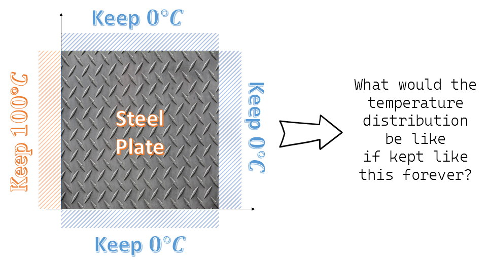
Figure 2. A physical phenomenon where the Laplace equation can be applied: steady state temperature
Let’s consider the problem of steady state temperature as one of the physical phenomena to which the Laplace’s equation can be applied. This problem can be thought of as finding out the temperature distribution inside a particular space after a long time has passed, given the temperature conditions on the boundary of that space, as shown in Figure 2.
The Laplace’s equation looks at this problem from the following perspective:
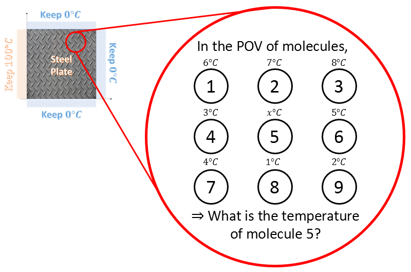
Figure 3. The perspective from which the Laplace's equation looks at the problem
In other words, the problem is about what temperature molecules that are not located at the boundary will have when the temperatures of the boundary are all determined, according to the Laplace equation. According to the Laplace equation, this molecule at position 5 will take the average of the temperatures of the surrounding molecules in the up, down, left, and right directions.
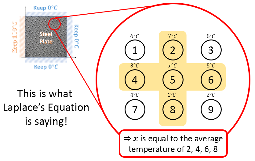
Figure 4. Perspective of the Laplace equation on the problem
Then, let’s explore the relationship between the second derivative coefficients, which make up the Laplace equation, and the average values of the surrounding molecules.
Another Meaning of the Second Derivative Coefficients: Average with Surrounding Values
In the previous section on heat equations/wave equations, we said that the second derivative coefficients represent the degree of “convexity” or “concavity.” However, it may be more helpful to think of the meaning of the second derivative coefficients as the “relationship with surrounding values” in a more comprehensive sense.
We want to confirm that the meaning of the second derivative coefficients also includes the “average value of surrounding values” by using Taylor series.
Taylor Series
※ For those in a hurry, you can just check equations (13) and (14) and move on.
In calculus, Taylor series is a method of representing an analytic function as an infinite sum of terms calculated from the values of its derivatives at a single point.

Figure 5. Process of approximating y=e^x at x=0 using Taylor series.
Source: Taylor Series, Wikipedia
Figure 5 illustrates the process of approximating $y=e^x$ at $x=0$ using Taylor series.
$y=e^x$ can be approximated using Taylor series as follows:
\[f(x) = e^x = \frac{x^0}{0!} + \frac{x^1}{1!} + \frac{x^2}{2!}+ \frac{x^3}{3!} + \cdots = \sum_{n=0}^{\infty}x^n\]The key point is that the original function, which is a transcendental function, can be represented as a polynomial function.
The definition of Taylor series is as follows.
| DEFINITION 1. Taylor Series |
|---|
$$T_f(x) = \sum_{n=0}^{\infty}\frac{f^{(n)}(a)}{n!}(x-a)^n \notag$$ $$=f(a) + f'(a)(x-a) + \frac{1}{2}f''(a)(x-a)^2 + \frac{1}{6}f'''(a)(x-a)^3 +\cdots $$ |
Using the definition of Taylor series from DEFINITION 1, let’s try to approximate $f(x)$ at a point $x_0$.
\[f(x) = f(x_0) + f'(x_0)(x-x_0) + \frac{1}{2}f''(x_0)(x-x_0)^2+\frac{1}{6}f'''(x_0)(x-x_0)^3+\cdots\]Let’s call the terms involving polynomials of degree 3 or higher as $R_3(x)$. In other words,
\[Equation (4) = f(x_0)+f'(x_0)(x-x_0)+\frac{1}{2}f''(x_0)(x-x_0)^2 + R_3(x)\]Now, for a sufficiently small positive real number $\Delta x$,
the value of the function $f(x)$ at the point $x_0+\Delta x$ is given by $f(x_0+\Delta x)$.
This can be obtained by substituting $x_0+\Delta x$ into equation (5).
\[f(x_0+\Delta x) = f(x_0) + f'(x_0)(x_0+\Delta x - x_0) + \frac{1}{2}f''(x_0)(x_0+\Delta x - x_0)^2 +R_3(x_0+\Delta x)\]Similarly, if we substitute $x-\Delta x$ into equation (5) instead of $x$, we get,
\[f(x_0-\Delta x) = f(x_0) + f'(x_0)(x_0-\Delta x - x_0) + \frac{1}{2}f''(x_0)(x_0-\Delta x - x_0)^2 +R_3(x_0-\Delta x)\]Now, adding equation (6) and equation (7) together, we obtain the following result.
\[f(x_0+\Delta x) + f(x_0-\Delta x) = 2f(x_0) + f''(x_0)(\Delta x)^2 + R_3(x_0+\Delta x) + R_3(x_0-\Delta x)\]Since we assume that $\Delta x$ is sufficiently small, we can consider $R_3(x_0+\Delta x) + R_3(x_0-\Delta x)$ in equation (8) as the error term and ignore the error.
Then, we can interpret equation (8) as follows.
\[f(x_0+\Delta x)+ f(x_0-\Delta) \approx 2f(x_0) + f''(x_0)(\Delta x)^2\]When we move the right-hand side of equation (9) to the left-hand side, we get:
\[f(x_0 + \Delta x) - 2f(x_0) + f(x_0-\Delta x) \approx f''(x_0)(\Delta x)^2\]In other words,
\[Equation (10) \Rightarrow \frac{f(x_0 + \Delta x) - 2f(x_0) + f(x_0-\Delta x)}{(\Delta x)^2} \approx f''(x_0)\]For equation (11), we can verify that the following holds for any arbitrary $x$ instead of $x_0$:
\[f''(x) = \frac{(x + \Delta x) - 2f(x) + f(x-\Delta x)}{(\Delta x)^2}\]If $f(x)$ was a multivariable function $u(x,y)$ instead, the following would also hold:
\[\frac{\partial^2 u}{\partial x^2}\approx \frac{u(x+\Delta x, y)-2u(x,y)+u(x-\Delta x, y)}{(\Delta x)^2}\] \[\frac{\partial^2 u}{\partial y^2}\approx \frac{u(x, y +\Delta y)-2u(x,y)+u(x, y-\Delta y)}{(\Delta y)^2}\]Back to the Laplace equation!
Let’s substitute the approximations of the second derivative coefficients from equations (13) and (14) into the Laplace equation we are trying to understand, which is as follows:
\[\frac{\partial^2 u}{\partial x^2} + \frac{\partial^2 u}{\partial y^2} = 0\]Let’s substitute the approximations of the second derivatives from equations (16) and assume $\Delta x = \Delta y$ for convenience. Then, equation (16) becomes:
\[u(x+\Delta x,y) - 2u(x,y) + u(x-\Delta x, y) + u(x, y+\Delta y) - 2u(x,y) + u(x, y-\Delta y) = 0\]Rearranging equation (17), we get:
\[4u(x,y) = u(x+\Delta x, y) + u(x-\Delta x, y) + u(x, y+\Delta y) + u(x,y-\Delta y)\]In other words,
\[u(x,y) = \frac{1}{4}\left\{ u(x+\Delta x, y) + u(x-\Delta x, y) + u(x, y+\Delta y) + u(x, y-\Delta y) \right\}\]What is equation (19) saying? It means that the temperature at point $u(x,y)$ is the average of the temperatures at four neighboring points. (Here, the neighboring points are separated by a distance of $\Delta x = \Delta y$.)
MATLAB Simulation
When we run a simulation of the example shown in Figure 2 using MATLAB, we obtain the following results.
It is important to note that the Laplace equation does not have an initial condition, but in the MATLAB simulation, the solution appears to change over time due to the iterative method used to obtain the solution. However, the actual solution according to the Laplace equation is shown in the final scene of the simulation.
Figure 6. Solution of the Laplace equation for the example shown in Figure 2