What is Gauss-Jordan Elimination?
Gauss-Jordan elimination is one of the methods for solving systems of linear equations.
This method is based on the principle that the solutions of the equations remain unchanged even after performing the following operations on the system of equations:
- Scaling each equation by a non-zero constant
- Adding or subtracting equations from each other
- Permuting the order of equations
In simpler terms, Gauss-Jordan elimination can be thought of as a process of using these three operations to transform the system of equations into the form $Ax=b$, where the matrix A can eventually become a unit matrix [1,0;0,1].
Let’s first perform Gauss-Jordan elimination through an example problem.
Gauss-Jordan Elimination through Example Problem
We want to find the solutions to the following system of equations:
\[\begin{cases}2x+2y = 2 \\4x+2y = 2\end{cases}\]1. Convert the given system of equations into matrix form
First, in order to use Gauss-Jordan elimination, we need to convert the given system of equations into the form $Ax=b$.
So, equation (1) can be written as follows:
\[\begin{bmatrix}2 & 2 \\4 & 2\end{bmatrix}\begin{bmatrix}x\\y\end{bmatrix}=\begin{bmatrix}2\\2\end{bmatrix}\]2. Combine matrix A and b into augmented matrix form
\[\left[\begin{array}{cc|c} 2&2&2\\ 4&2&2\end{array}\right]\]3. Scaling (row1 -> row1 x 1/2)
We multiply row1 by 1/2 so that the first number in row1 becomes 1.
\[\left[\begin{array}{cc|c} 2&2&2\\ 4&2&2\end{array}\right] \longrightarrow \left[\begin{array}{cc|c} 1&1&1\\ 4&2&2\end{array}\right]\]4. Subtraction (row2 -> row2 - 4 x row1)
We subtract 4 times row1 from row2 so that the first number in row2 becomes 0.
\[\left[\begin{array}{cc|c} 1&1&1\\ 4&2&2\end{array}\right] \longrightarrow \left[\begin{array}{cc|c} 1&1&1\\ 0&-2&-2\end{array}\right]\]5. Scaling (row2 -> row2 x (-1/2))
We multiply row2 by (-1/2) so that the second number in row2 becomes 1.
\[\left[\begin{array}{cc|c} 1&1&1\\ 0&-2&-2\end{array}\right] \longrightarrow \left[\begin{array}{cc|c} 1&1&1\\ 0&1&1\end{array}\right]\]6. Subtraction (row1 -> row1 - row2)
We subtract row2 from row1 so that the second number in row1 becomes 0.
\[\left[\begin{array}{cc|c} 1&1&1\\ 0&1&1\end{array}\right] \longrightarrow \left[\begin{array}{cc|c} 1&0&0\\ 0&1&1\end{array}\right]\]Solution!
After going through these 6 steps, we can determine that the solution to the system of equations in equation (1) is:
\[(x,y) = (0,1)\notag\]The Geometric Meaning of Gaussian Elimination
Let’s visualize the process of solving equation (1) using the Gaussian-Jordan matrix elimination method.
Geometrically, the Gaussian-Jordan matrix elimination method is the process of transforming the normal vectors of a line equation into unit vectors parallel to each other. (The intersection point should not change during this process.)
Equation (1) can be thought of as a problem of solving simultaneous equations, but it can also be thought of as a problem of finding the intersection point of two linear functions.
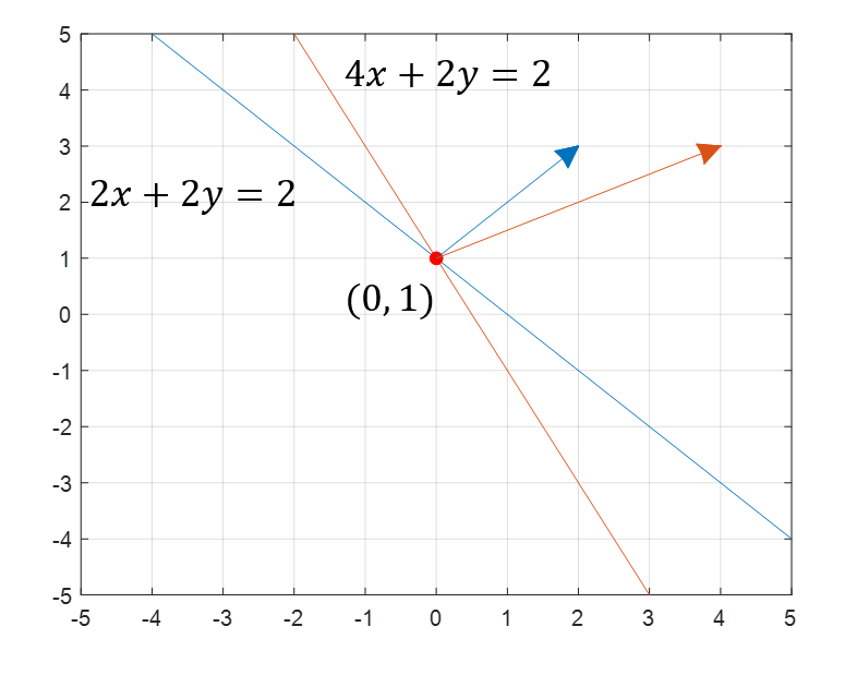
Figure 1. A representation of equation (1) as a problem of finding the intersection point of two functions on the Cartesian plane.
In Figure 1, we have shown the two functions corresponding to the simultaneous equation (1) and their intersection point.
The blue and orange lines in Figure 1 represent the functions corresponding to $2x+2y=2$ and $4x+2y=2$, respectively.
We can also see the normal vectors of the two functions in Figure 1. The normal vectors corresponding to $2x+2y=2$ and $4x+2y=2$ are shown in blue and orange, respectively, and their vector values are (2,2) and (4,2), respectively.
So, let’s try to visually understand what the Gaussian-Jordan matrix elimination method is.
Step-by-Step Visualization of the Same Example Problem
1. Visualize the given simultaneous equation as two linear functions
We can visualize the given simultaneous equation as two linear functions, as shown in Figure 1.
2. (Change to an augmented matrix form by combining matrix A and b)
This step is not part of the visualization process, so it is omitted.
3. Scaling (row1 -> row1 x 1/2)
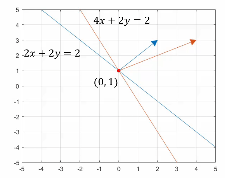
Figure 2. Visualization of the process of multiplying the first equation of equation (1) by 1/2 using scaling.
Scaling has the effect of reducing the size of the normal vector or changing its direction.
In this scaling step, we multiply the first equation of equation (1) by 1/2, and as shown in Figure 2, it has the effect of reducing the size of the normal vector.
Note that the first element of the transformed normal vector has changed from 2 to 1 in this step.
4. Subtraction (row2 -> row2 - 4 x row1)
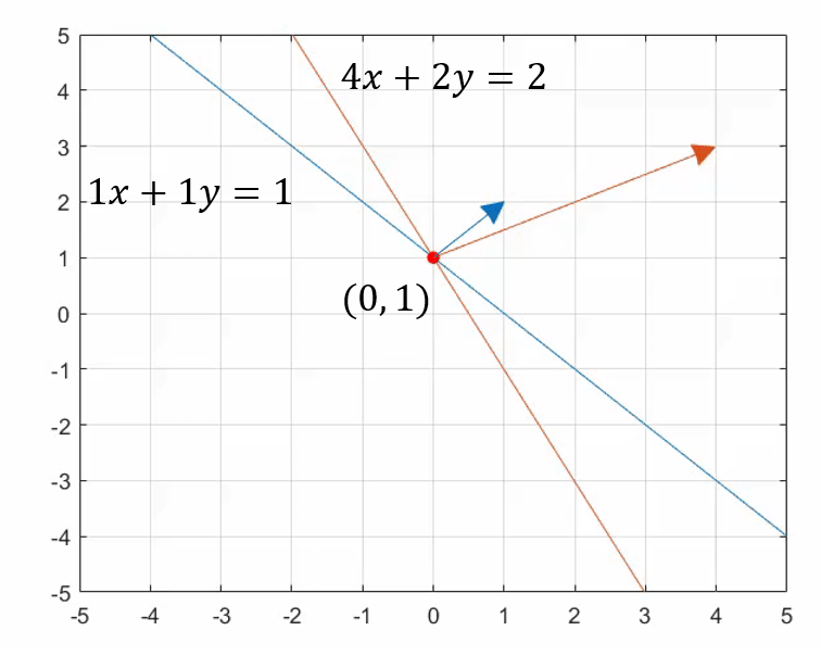
Figure 3. Visualization of the process of making the normal vector of the second equation in Equation (1) parallel to the y-axis through the subtraction process.
Through the subtraction process, one of the two elements of a 2-dimensional vector becomes zero, and the normal vector is transformed to be parallel to the x-axis or y-axis. Figure 3 shows the process of transforming the normal vector of the second equation in Equation (1) to be parallel to the y-axis through the subtraction process.
5. Scaling (row2 -> row2 x (-1/2))
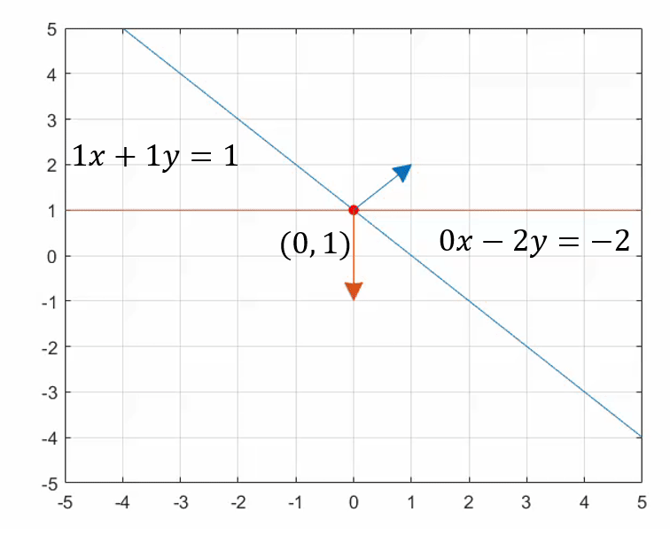
Figure 4. Visualization of the process of making the normal vector of the second equation in Equation (1) parallel to the y-axis while maintaining the same direction through the scaling process.
In Figure 4, the scaling process is used to make the normal vector of the second equation in Equation (1) parallel to the y-axis while maintaining the same direction as the unit vector.
6. Subtraction (row1 -> row1 - row2)
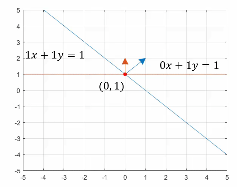
Figure 5. Visualization of the process of making the normal vector of the first equation in Equation (1) parallel to the x-axis while maintaining the same direction through the subtraction process.
Through the subtraction process, one of the two elements of a 2-dimensional vector becomes zero, and the normal vector is transformed to be parallel to the x-axis or y-axis. Figure 5 shows the process of transforming the normal vector of the first equation in Equation (1) to be parallel to the x-axis through the subtraction process.
Solution!
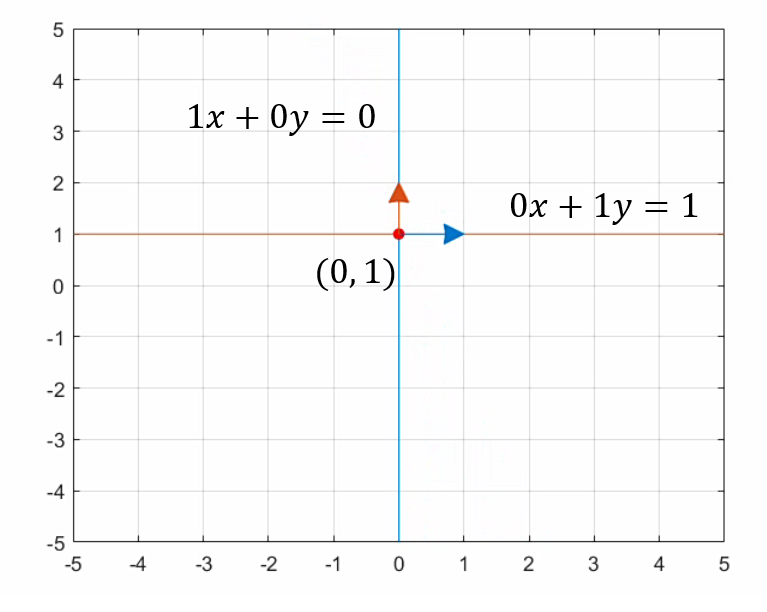
Figure 6. The final result obtained through the Gauss-Jordan elimination method for the transformed normal vectors and the solutions of the system of equations.
Figure 6 shows the final result obtained through the Gauss-Jordan elimination method. As we can see from the process shown in Figures 1 to 5, the solutions of the system of equations remain unchanged, but the normal vectors are transformed.
In summary, the Gauss-Jordan elimination method can be described as a process of transforming the normal vectors of linear equations to be parallel to the unit vectors (or basis vectors) through linear transformations. By going through this process, we can obtain the solutions more conveniently.
Visualization of 3-Dimensional Cases
In the case of three variables, $x, y, z$, and three simultaneous equations, it is also possible to visualize the process. However, visualizing 3-dimensional cases can be challenging to understand at a glance, so I will omit detailed explanations and show only the animated visualization.
In the animation, I have visualized the process of finding solutions for the following system of simultaneous equations:
\[\begin{cases}10x+10y+15z = 2 \\3x-2y+4z = 4 \\-4x+4y+5z=1\end{cases}\]The blue, orange, and yellow colors represent the first, second, and third equations, respectively.