1. Definition of Laplacian
In Euclidean space, the Laplacian is defined as the divergence of the gradient of a scalar function $f$ that can be twice differentiable. It can be mathematically expressed as follows:
\[\Delta f = \nabla ^2 f = \nabla \cdot \nabla f\]Although it may seem complicated mathematically, let’s try to understand the intuitive meaning of the Laplacian.
2. Gradient and Divergence of Scalar Functions
Simply put, the Laplacian for a scalar function can be understood as the divergence of the gradient operation applied to the function:
\[div(grad(f))\]Consider the following scalar function. It is a beautiful scalar function that can be created using the “peak” function in MATLAB.
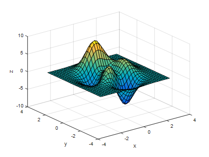
Figure 1. Plot of the "peak" function in MATLAB. What would be its gradient?
Figure 1 shows the plot of the “peak” function in MATLAB.
What can we predict about the gradient of this scalar function?
The gradient represents the direction of steepest increase, and a vector field is formed in the direction of the steepest slope. It may sound ambiguous when explained in words, but let’s try to imagine what vector field would be formed.
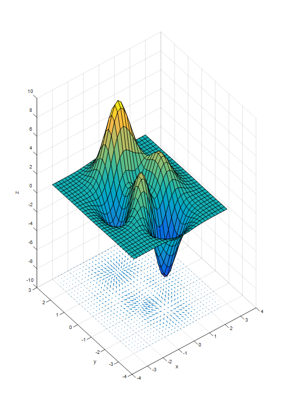
Figure 2. The "peak" function and its gradient displayed.
The z-coordinate of the vector field in Figure 2 being -10 is arbitrarily chosen in order to depict the peak function and vector field together.
As we can see from Figure 2, near the (0, 2) coordinates, a vector field is converging to a single point, while near the (0, -2) coordinates, a vector field is diverging from a single point.
Now, what would happen if we calculate the divergence of this vector field?
Since the vector field is converging near (0, 2), the divergence would be negative, and since it is diverging near (0, -2), the divergence would be positive.
In other words, taking the gradient of a scalar function and then taking the divergence of it is similar to showing numerically how low or high the height value of that scalar function is.
Let’s confirm if this statement is true by plotting the grad($f$) on a 2D plane, as shown in Figure 3.
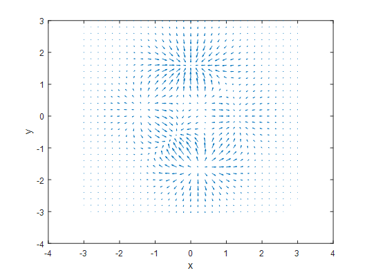
Figure 3: Gradient of the peak function plotted on the xy plane.
Figure 3 shows the vector field from Figure 2 translated to the xy plane. Now, let’s calculate the divergence and visualize it using colors.
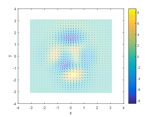
Figure 4: Divergence applied to the vector field in Figure 3 and visualized with colors.
As I mentioned earlier, since divergence indicates how low or high the height of a scalar function is, the reciprocal of divergence represents how high the height of the function is.
From Figures 5 and 6, we can see that the negative values of divergence indeed closely resemble the height of the peak function.
In reality, the Laplacian indicates the value of the second partial derivative. In other words, the Laplacian tells us if a scalar function is concave downwards ($\nabla^2f>0$) or concave upwards ($\nabla^2f<0$) at that point.
This is the same interpretation as the meaning of the second derivative coefficients that we learned in high school.