Prerequisites
To understand this post, it is recommended that you are familiar with the following topics:
- Basic operations of vectors
- A new perspective on matrix multiplication
- Geometric meaning of Euler’s formula
What is Fourier Transform?
The Fourier transform is used when analyzing the frequency components of a signal.
To give a simple example, let’s say a low-pitched man and a high-pitched woman are speaking at the same time.
The sound we hear will be a mixture of low and high frequencies.
Here are the pieces of information we want to know:
- What are the frequencies of the low and high pitches? (In other words, how high or low are they in numerical terms?)
- What is the relative signal magnitude ratio between the low and high pitches? (In other words, how loud were their voices?)
Example of using Fourier Transform
Let’s take a more concrete example of a signal and its Fourier transform analysis using the previous example.
In Figure 1 below, a signal consisting of a 50Hz sine wave and a 120Hz sine wave is depicted.
That is, a low-frequency signal and a high-frequency signal are combined, with amplitudes of 0.7 and 1, respectively.
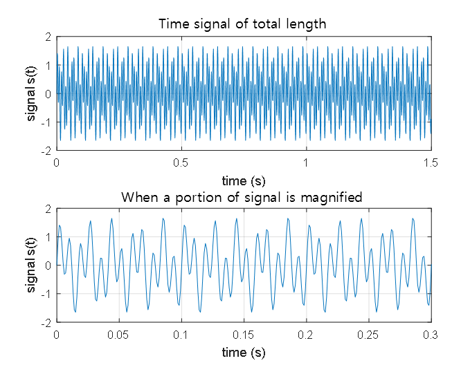
Figure 1. A signal consisting of a 50Hz sine wave and a 120Hz sine wave
Suppose we received a signal like Figure 1 without any background information.
In other words, can we identify the components of the entire signal, such as the frequency values of the low and high pitches and the relative signal magnitude ratio between them?
We can apply the Fourier transform to obtain the components of the signal, as shown below.
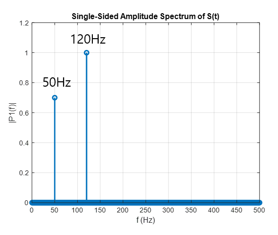
Figure 2. The Fourier transform result shows that the signal contains two frequency components, 50Hz and 120Hz.
Signals can also be viewed as vectors.
So what is the relationship between the linear algebra and Fourier transform that we have studied so far?
The most important concept is that “signals can also be viewed as vectors.”
What does this mean?
In the Basic Operations of Vectors post, we introduced the perspective that “a vector is a sequence of numbers listed in order.”
Let’s think again that the voice signal introduced in the previous example is just a list of numbers obtained by converting the pressure of the sound obtained through a recording device into a sequence.
For example, suppose we record our voice signal through a microphone that can acquire 1 data per second from the sound waveform.
When we record for a total of 10 seconds, the acquired data can be expressed as a list of 10 numbers.
If the performance of this microphone is good enough to acquire 100 data per second, the acquired data for 10 seconds can be expressed as a list of 1000 numbers.
(Actually, the latest recording devices can acquire more than 40,000 data per second!)
That is, if we express the recorded signal as a vector, it can be written as follows.
If the total length of the data is $N$,
\[x[n] = \begin{bmatrix}x[0]\\x[1] \\ \vdots \\ x[N-1]\end{bmatrix}\]As introduced in the Basic Operations of Vectors post, since the basic operations (scalar multiplication and vector addition) are satisfied for voice signals, voice signals can also be viewed as a type of vector, and the dimension of the $x[n]$ vector is $N$.
Frequency components can also be viewed as vectors.
So, what about the frequency components we saw in Figure 2?
Frequency components can also be viewed as vectors.
This part may sound somewhat difficult, but,
Suppose the first element of the frequency component vector represents the component value of 0Hz, and the second element represents the component value of 1Hz, etc.
In this way, if we divide the appropriate frequency bands into $N$ parts, the frequency component can also be represented as a vector.
If we divide the entire frequency band into $N$ parts, just like the length of the time signal, the frequency component vector can also be represented as follows.
\[X[k] = \begin{bmatrix}X[0]\\X[1]\\ \vdots \\ X[N-1] \end{bmatrix}\]Fourier Transform: Linear Transformation between Time Signal Vectors and Frequency Signal Vectors
※ This excerpt is taken from Frequency Sampling and DFT.
In our new perspective on matrix multiplication, we learned that matrices are functions (more specifically, linear transformations) that take vectors as input and output another vector.
But what did we do in Figure 2?
We transformed a time signal vector into a frequency vector.
In other words, we transformed one vector into another.
We can intuitively understand that there exists a matrix that can perform such a transformation.
We call this matrix the “Fourier matrix.”
The Fourier matrix can be obtained from the following discrete Fourier transform:
| DEFINITION: DFT and iDFT |
|---|
| For a discrete signal $x[n]$ of length N and its discrete frequency component $X[k]$ of length N, |
We can think of obtaining a frequency component vector from a signal vector by multiplying it with a matrix (in this case, the Fourier matrix). To see this, let’s calculate the values of $X[k]$ for $k=0,1,\cdots, N-1$.
\[X[0] = x[0]\exp\left(-j\frac{2\pi 0}{N}0\right) + x[1]\exp\left(-j\frac{2\pi 0}{N}1\right)+\cdots +x[N-1]\exp\left(-j\frac{2\pi 0}{N}(N-1)\right)\] \[=x[0]\cdot 1 + x[1]\cdot 1 + \cdots + x[N-1] \cdot 1\] \[X[1] = x[0]\exp(\left(-j\frac{2\pi 1}{N}0\right)+x[1]\exp\left(-j\frac{2\pi 1}{N}1\right)+\cdots +x[N-1]\exp(\left(-j\frac{2\pi 1}{N}(N-1)\right)\]For simplicity of notation, let’s define
\[w = \exp\left(-j\frac{2\pi}{N}\right)\]Then,
\[X[1]\Rightarrow x[0]w^0 + x[1] w^1 + \cdots + x[N-1]w^{N-1}\]We can calculate the $i$th frequency component $X[i]$ as follows:
\[X[i] = x[0]w^0 + x[1]w^{i\times1}+\cdots+x[j]w^{i\times j}+\cdots +x[N-1]w^{i\times(N-1)}\]Therefore, we can express the DFT as a relationship between a vector and a matrix through this process as follows:
\[\begin{bmatrix}X[0]\\X[1]\\ \vdots \\ X[N-1]\end{bmatrix} = \begin{bmatrix} 1 && 1 && 1 && \cdots && 1 \\ 1 && w^1 && w^2 && \cdots && w^{N-1} \\ \vdots && \vdots && \vdots && \ddots && \vdots \\ 1 && w^{N-1} && w^{(N-1)\cdot 2} && \cdots && w^{(N-1)\cdot(N-1)}\end{bmatrix}\begin{bmatrix}x[0]\\x[1]\\ \vdots \\ x[N-1]\end{bmatrix}\]In the article Matrix as Linear Transformation, it is mentioned that matrices are a kind of linear transformation, and in the article Another Perspective on Matrix Multiplication, it is explained that the multiplication of matrices is the inner product between a row of the matrix on the left and a column of the matrix on the right.
The meaning of the inner product is “similarity,” and multiplying the Fourier matrix by a signal vector means obtaining the frequency component by checking how similar the rows of the Fourier matrix are to the signal vector.
So, what is the meaning the Fourier matrix?
In the article Geometric Interpretation of Euler’s Formula, the meaning of the following formula is explained:
\[e^{j\theta}=\cos(\theta) + j\sin(\theta)\]To understand the meaning of Equation (12), we can see that the value on the right side represents the coordinates of the arc rotated counterclockwise by $\theta$ radians from the origin in the complex plane.
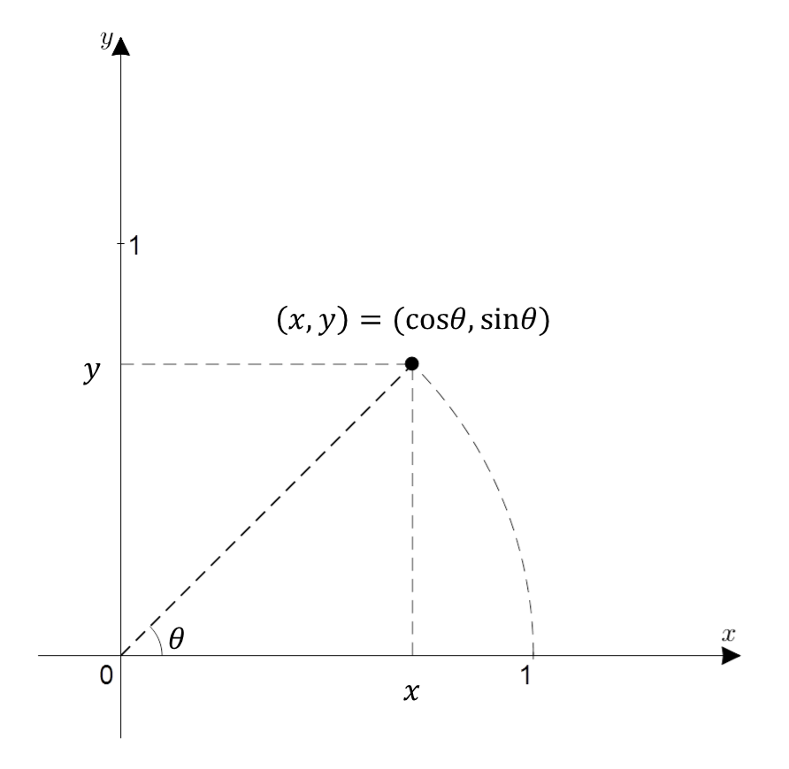
Figure 4. $x+iy$ represented on the complex plane. When expressed in trigonometric functions, it is $\cos\theta + i \sin\theta$, where $\theta$ is the angle from the $x$-axis measured in radians.
In other words, $w$ in equation (8) is calculated as follows:
\[w = \exp\left(-j\frac{2\pi}{N}\right)\]This means that $w$ is the position of the first point that divides a circle into $N$ equal parts and rotates clockwise once.
Let’s take the example of the Fourier matrix with $N=8$ and examine the meaning of $w$ while considering its value.
For $N=8$, the value of $w$ in the Fourier matrix is $w=\exp\left(-j\frac{2\pi}{8}\right)$. If we represent this on the complex plane, it looks like this:
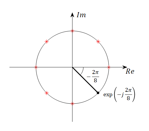
Figure 5. $\exp(-j 2\pi/8)$ represented on the complex plane. The red asterisks indicate $w^0, w^2, w^3, ..., w^7$.
If we replace the complex numbers inside the Fourier matrix with the phases indicated by the complex number $w$ on the unit circle of the complex plane, it would look like Figure 6 below.
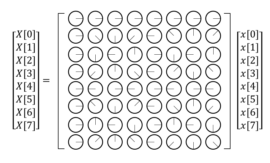
Figure 6. Visualization of the Fourier matrix for $N=8$. The figures inside the matrix represent the phases indicated by the complex number $w$ on the unit circle of the complex plane.
Since both cosine and sine functions originate from the rotation of a circle, we can think of the values of the phase as being replaced by the values of the cosine or sine function.
Therefore, if we consider the phase in the Fourier matrix with respect to the cosine function, we can think of it as follows:
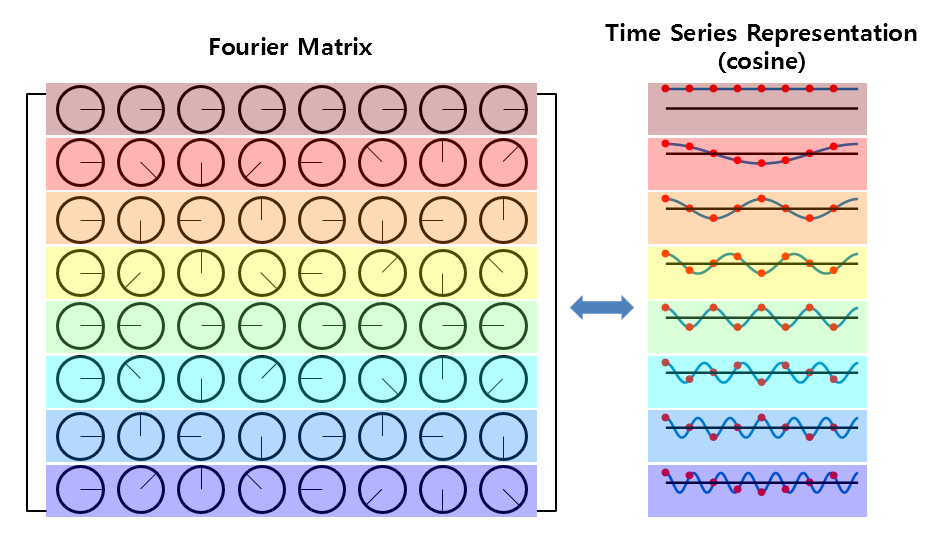
Figure 7. When we replace the phase of each complex number in the Fourier matrix with the value of the cosine function.
As shown in Figure 7 above, each row of the Fourier matrix represents a cosine function from frequency 0 to multiples of the fundamental frequency.
Also, considering the phase of the Fourier matrix for the sine function, as shown in Figure 8 below,
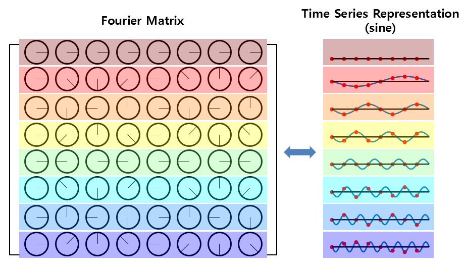
Figure 8. Replacing the phase of each complex element in the Fourier matrix with a sine function.
As shown in Figure 8 above, each row of the Fourier matrix also represents a sine function from frequency 0 to multiples of the fundamental frequency.
In other words, the Fourier matrix used to calculate the DFT is composed of cosine and sine functions that are multiples of the fundamental frequency. These functions make up the real and imaginary parts and are multiplied by the original time signal to obtain the result.
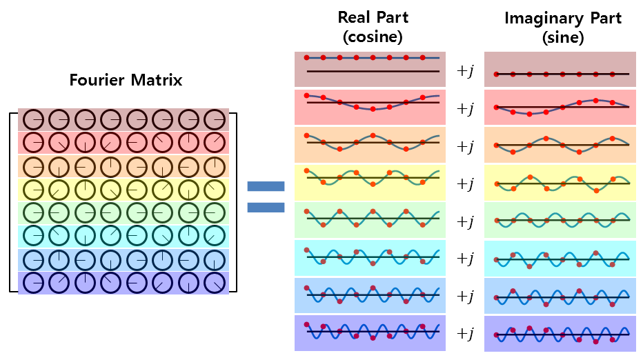
Figure 9. All values in the Fourier matrix are complex numbers, and the real and imaginary parts are composed of cosine and sine functions, respectively.
Characteristics of the Fourier Matrix
Now let’s look at the characteristics of the Fourier matrix.
1. The columns of the Fourier matrix are orthogonal to each other.
We can easily confirm that each column of the Fourier matrix is orthogonal to each other.
The easiest way to do this is to take the Hermitian operation on the Fourier matrix $F$ and multiply it.
That is,
\[F^HF = \begin{bmatrix} 1 && 1 && 1 && \cdots && 1 \\ 1 && w^{*1} && w^{*2} && \cdots && w^{*(N-1)} \\ \vdots && \vdots && \vdots && \ddots && \vdots \\ 1 && w^{*(N-1)} && w^{*(N-1)\cdot 2} && \cdots && w^{*(N-1)\cdot(N-1)}\end{bmatrix}\times\notag\] \[\begin{bmatrix} 1 && 1 && 1 && \cdots && 1 \\ 1 && w^1 && w^2 && \cdots && w^{N-1} \\ \vdots && \vdots && \vdots && \ddots && \vdots \\ 1 && w^{N-1} && w^{(N-1)\cdot 2} && \cdots && w^{(N-1)\cdot(N-1)}\end{bmatrix}\] \[=N\begin{bmatrix}1 && 0 && \cdots && 0 \\ 0 && 1 && \cdots && 0 \\ \vdots && \vdots && \ddots && \vdots \\ 0 && 0 && \cdots && 1\end{bmatrix} = N\cdot I\]Here, the superscript ‘*’ denotes complex conjugate.
To verify this, consider the m-th row and n-th column of the calculation result of $F^HF$.
\[F^H_{m,:}F_{:,n} = \begin{bmatrix}1 & w^{*\cdot m \cdot 1} & \cdots & w^{*\cdot m \cdot (N-1)}\end{bmatrix}\cdot \begin{bmatrix}1\\w^{1\cdot n} \\ \vdots \\ w^{(N-1)\cdot n}\end{bmatrix}\] \[=1+w^{*\cdot m\cdot 1}w^{1\cdot n}+\cdots+w^{*\cdot m\cdot (N-1)}w^{(N-1)\cdot n}\] \[=\sum_{k=0}^{N-1}w^{*m\cdot k}w^{k\cdot n}\] \[=\sum_{k=0}^{N-1}\exp\left(j\frac{2\pi}{N}m\cdot k\right)\exp\left(-j\frac{2\pi}{N}n\cdot k\right)\] \[=\sum_{k=0}^{N-1}\exp\left(j\frac{2\pi}{N}(m-n)\cdot k\right)\]Therefore, when $m=n$, $F^H_{m,:}F_{:,n}=N$ and when $m\neq n$, $F^H_{m,:}F_{:,n}=0$.
As in the result of equation (15), each column of the Fourier matrix $F$ has a value of $N$ when the column itself is inner-producted and 0 when inner-producted with other columns, so we can see that each column is orthogonal to each other.
2. Inverse Fourier Matrix and Inverse Fourier Transform
Also, from equations (14) and (15), we can see that the inverse matrix of the Fourier matrix is
\[F^{-1}=\frac{1}{N}F^H\]That is,
\[\begin{bmatrix}x[0]\\x[1]\\ \vdots \\ x[n-1]\end{bmatrix} = \frac{1}{N}\begin{bmatrix} 1 && 1 && 1 && \cdots && 1 \\ 1 && w^{*1} && w^{*2} && \cdots && w^{*(N-1)} \\ \vdots && \vdots && \vdots && \ddots && \vdots \\ 1 && w^{*(N-1)} && w^{*(N-1)\cdot 2} && \cdots && w^{*(N-1)\cdot(N-1)}\end{bmatrix}\begin{bmatrix}X[0]\\X[1]\\ \vdots \\ X[N-1]\end{bmatrix}\]and this is the same as the equation for the inverse DFT.
3. What the Inverse Fourier Transform Tells Us
Let’s revisit the analysis part based on the column space from A New Perspective on Matrix Multiplication.
For example, for the following matrix,
\[\begin{bmatrix}1 & 2 \\ 3 & 4\end{bmatrix}\begin{bmatrix}x\\y\end{bmatrix}=\begin{bmatrix}3\\5\end{bmatrix}\]Solving simultaneous equations can be easily done as shown below.
\[\begin{cases}x+2y = 3 \\3x+4y = 5\end{cases}\] \[\Rightarrow x=-1, \text{ }y=2\]However, let’s think of this equation in the following way.
\[x\begin{bmatrix}1\\3\end{bmatrix}+y\begin{bmatrix}2\\4\end{bmatrix}=\begin{bmatrix}3\\5\end{bmatrix}\]As mentioned in A New Perspective on Matrix Multiplication, the above equation can also be interpreted as follows:
If we apply this idea directly to Fourier matrices, the meaning of taking the inverse Fourier transform is as follows:
“Does a N-dimensional time series vector exist in the vector space generated by the N columns of $F^{-1}$?”
“If so, how can we combine the column vectors of $F^{-1}$ to create the time series vector?”
In other words,
“All time series can be represented as a sum of sine waves, and the form of the time series is determined by how we combine the sine waves.”