Prerequisites
To better understand the meaning of non-homogeneous differential equations, it is recommended to have knowledge about the following topics.
- Direction Fields and Euler’s Method
- Solutions to First-Order Linear Differential Equations
- Modeling with Systems of Differential Equations
- Phase Plane
First-Order Non-homogeneous Differential Equations
The general form of a first-order linear differential equation is:
\[\frac{dx}{dt}+p(t)x=q(t)\]If $q(t)=0$, we call the equation homogeneous, and if $q(t)\neq0$, we call it non-homogeneous.
(Here, “DE” stands for “differential equation”. In this article, we will use the terms “homogeneous” and “non-homogeneous” among the Korean expressions.)
However, when studying differential equations, we do not spend much time discussing first-order non-homogeneous differential equations. This is because finding solutions to these equations is not difficult.
As we learned in the solutions to first-order linear differential equations, the solution to a first-order non-homogeneous differential equation such as equation (1) can be expressed as follows:
Consider a function $\mu(t)$ such that $\int p(t)dt = \mu(t)$, then
\[x(t) = \frac{1}{e^{\mu(t)}}\left(\int e^{\mu(t)}q(t)dt + C\right)\]However, if we only focus on how to find solutions to homogeneous and non-homogeneous differential equations, we may not fully understand the meaning of non-homogeneous differential equations.
Non-homogeneous differential equations differ from homogeneous differential equations in that they involve a term that is dependent only on the independent variable added to the rate of change of $x$.
For example, the following differential equation is a homogeneous differential equation:
\[\frac{dx}{dt} = x\]However, some differential equations can be expressed in the form below, as the change in $x(t)$, the rate of change of $dx/dt$, can also vary with respect to the independent variable $t$.
\[\frac{dx}{dt} = x+e^{t/2} % Equation (4)\]If we draw the direction fields and solution curves corresponding to Equations (3) and (4), we get Figure 1 below.
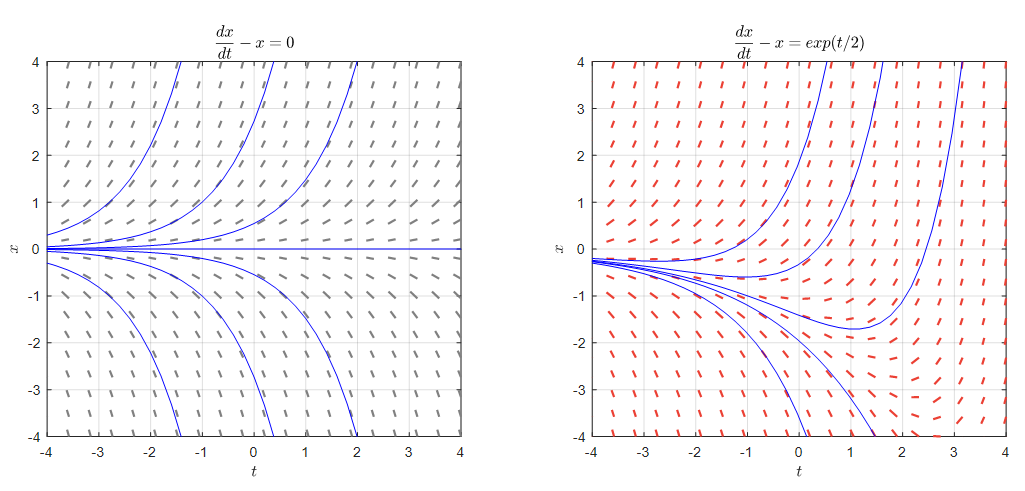
Figure 1. Comparison of direction fields of homogeneous/nonhomogeneous differential equations (corresponding to Equations (3) and (4))
Looking at the slopes of the two direction fields in Figure 1, it appears that the forms of the direction fields in the left and right graphs are not very different when the independent variable $t$ is less than 0. However, as $t$ increases, we can see that the form of the direction field changes significantly.
This is because the $\exp(t/2)$ function in Equation (4) increases in value as the independent variable $t$ increases, causing the slope values to change more significantly.
Referring back to Equation (1), a nonhomogeneous differential equation is essentially the form of the original homogeneous equation
\[\frac{dx}{dt}+p(t)x = 0 % Equation (5)\]with the addition of $q(t)$ to the right-hand side. In other words, a change that depends only on $t$ is added to the form of the direction field of the original homogeneous differential equation.
This is illustrated in Figure 2 below.
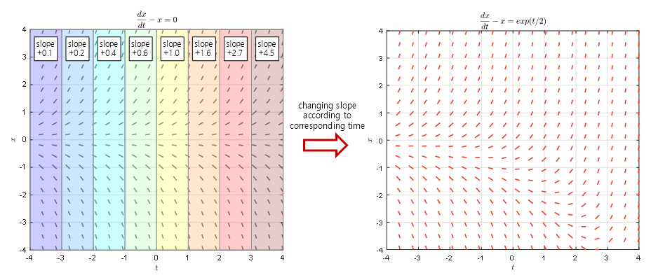
Figure 2. The direction field of a nonhomogeneous differential equation is obtained by adding the value of the nonhomogeneous term (i.e., $q(t)$ in Equation (1)) to the slope for each interval of the independent variable.
System of Non-Homogeneous Differential Equations
Let’s consider a system of differential equations with two or more equations when the equations are dependent on each other.
In the Modeling with System of Equations post, we introduced the homogeneous system of differential equations that can model the changes of two dependent variables simultaneously as follows:
\[\begin{cases}\dfrac{dx}{dt} = f(x,y) \\\\ \dfrac{dy}{dt}=g(x,y)\end{cases}\]If we transform the system of differential equations into non-homogeneous form, it can be represented as follows:
\[\begin{cases}\dfrac{dx}{dt} = f(x,y) + p(t)\\\\ \dfrac{dy}{dt}=g(x,y) + q(t)\end{cases}\]The system of non-homogeneous differential equations is similar to first-order non-homogeneous differential equations, as the rates of change of dependent variables $x$ or $y$ are affected by the values that depend only on the independent variable.
However, when trying to visualize the system of non-homogeneous differential equations, there is a problem. For instance, if we have a system of non-homogeneous differential equations with two dependent variables $x$ and $y$, there is no room for an independent variable $t$ in the horizontal and vertical axes of the phase plane.
The first way to visualize such systems is by using a three-dimensional plot. This method assigns one axis to the independent variable, and it draws the phase plane as the independent variable changes.
However, this method is not intuitive enough to understand the changes at a glance.
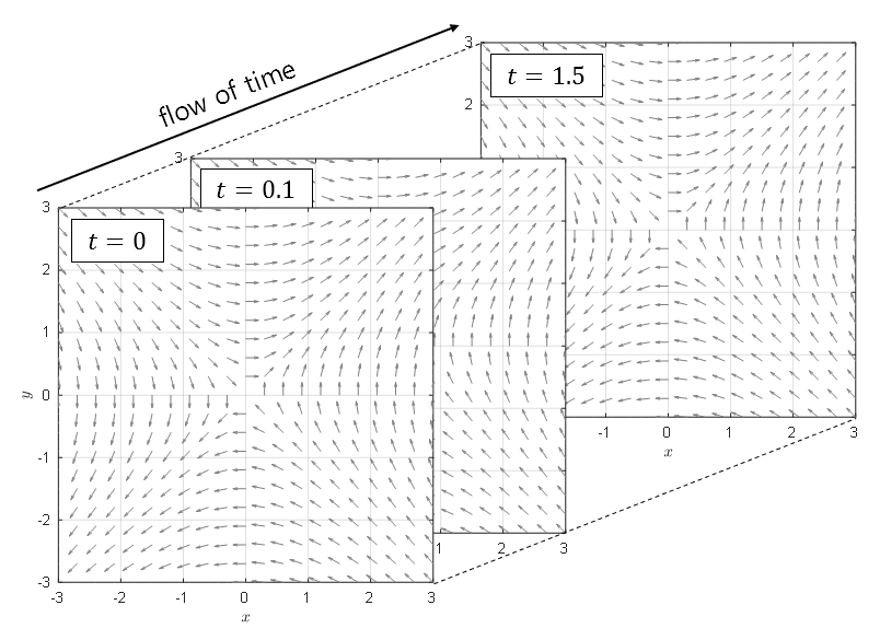
Figure 3. The shape of the phase plane represented in 3D with an added time axis. It is difficult to understand the changes at a glance.
The second way is to create an animation. In other words, we interpret the independent variable as time and draw the phase plane changes at each moment.
In other words, it is an animation.
We will use the second method to understand the characteristics of the solution to the system of non-homogeneous differential equations.
For example, consider the following second-order system of non-homogeneous differential equations:
\[\begin{cases}\dfrac{dx}{dt} = y + \cos(t)\\\\ \dfrac{dy}{dt}=x+\sin(t) \end{cases}\]In the homogeneous differential equation form of the equation above, there would be no term of $\cos(t)$ or $\sin(t)$, and the phase plane would look like the following:
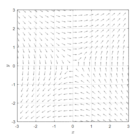
Figure 4. The phase plane representation of the homogeneous equation form of equation (8)
Now, if we add a time-dependent term of $\cos(t)$ or $\sin(t)$ to make the phase plane vary according to the value of $t$, it would look like the following:
Figure 5. The variation of the phase plane according to the time $t$ in equation (8)
The fact that the phase plane changes over time means that the direction in which the curve corresponding to the initial condition changes also changes constantly. This is illustrated in Figure 6 below.
Figure 6. The variation of the solution curve according to different initial conditions
For example, the solution curve starting from (2, -3) would be drawn as shown in the following video.
Figure 7. The solution curve corresponding to a specific initial condition
The reason why “General Solution = Homogeneous + Particular Solution”.
The reason why the general solution is the sum of the homogeneous solution and the particular solution is one of the most difficult concepts to understand when studying differential equations as an undergraduate.
I.e., the general solution of a differential equation is the sum of the homogeneous solution and the particular solution.
For example, if we solve the differential equation:
\[x''-4x'+3x=t % Equation (9)\]the general solution is:
\[x(t) = x_h(t) + x_p(t) = \left(c_1 e^t + c_2 e^{3t}\right) + \left(\frac{t}{3} + \frac{4}{9}\right) % Equation (10)\]where (the specific method for finding this solution will be explained later).
The first part,
\[x_h(t) = c_1 e^t + c_2 e^{3t} % Equation (11)\]is obtained by solving the homogeneous differential equation:
\[x''-4x'+3x=0 % Equation (12)\]The second part,
\[x_p(t) = \frac{t}{3}+\frac{4}{9} % Equation (13)\]is obtained by solving only Equation (9).
(In other words, it satisfies the original non-homogeneous differential equation when plugged in for $x_p(t)$.)
The two results in Equations (11) and (13) are each called the homogeneous solution and the particular solution, respectively.
At first glance, it may seem that the particular solution in Equation (13) alone is sufficient for the general solution, but in reality, it is $x(t) = x_h(t)+x_p(t)$.
The reason for this can be understood from Figure 1 or Figure 4, as the solution to a non-homogeneous differential equation is the addition of the slope change obtained from the independent variable-dependent function in the form of the direction field or phase plane of the original homogeneous differential equation.
Moreover, when we think about Figure 1 or Figure 5, it is impossible to think of a slope change based only on the non-homogeneous term dependent on the independent variable.
Therefore, the complete solution to a non-homogeneous differential equation must be thought of as the sum of the solutions to the homogeneous differential equation and the solution obtained from the non-homogeneous term.