Frequency Transformation

This post is a summary of Professor S. C. Duta Roy’s lecture at IIT (Indian Institute of Technology), which can be found at here.

Objectives

Understand the concept of Normalized Lowpass Filter.
Understand the transformation between filters.
Understand the geometrically symmetric property of Bandpass Filters or Bandstop Filters and the problems and solutions it brings.
Design filters using Butterworth and Chebyshev Filters based on filter specifications.

1. Frequency Transformation

a. Normalized Lowpass Filter

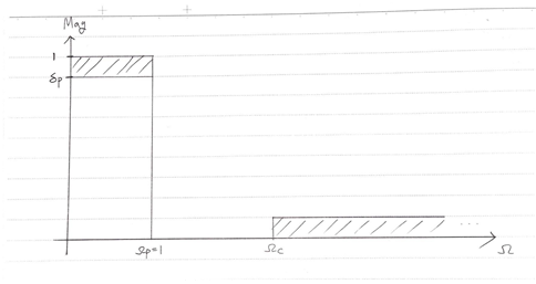
Figure 1. Normalized Lowpass Filter.

The Normalized Lowpass Filter (NLPF) is a type of Lowpass Filter with $\Omega_p=1$, and $\Omega_c$ is a variable that can be changed according to the filter’s specification. NLPF is important because it can be transformed into any other type of filter.

b. Terminology

For convenience, we will refer to other types of filters as Other Kinds of Filters (OKF), which are all denormalized forms of NLPF. We will also use the abbreviations LPF, HPF, BPS, and BSP for Lowpass, Highpass, Bandpass, and Bandstop Filters, respectively.

To distinguish between the Laplace frequency $s=j\Omega$ before and after transformation, we will use uppercase S for NLPF and lowercase s for the transformed form.

c. Frequency Transformation from NLPF to OKF

1) NLPF $\rightarrow$ Denormalized LFP

The transformation from Normalized Lowpass Filter (NLPF) to Denormalized Lowpass Filter (DLPF) is generally achieved by the following transformation:

Definition 1. Transformation

Normalized Lowpass Filter $\rightarrow$ Denormalized Lowpass Filter

To obtain a Denormalized Lowpass Filter with a passband frequency $\Omega_p$ from a Normalized Lowpass Filter, the following transformation can be applied:

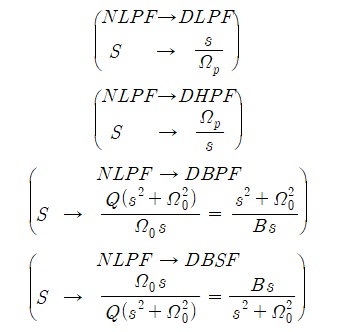
\[S\rightarrow \frac{s}{\Omega_p}\]

In summary, the statement “transform $S$ to $s/\Omega_p$” means that $S$ should be replaced by $s/\Omega_p$.

This transformation is not difficult, but it demonstrates the validity of frequency transformation. For example, the transformation can be achieved through the following process. Consider a simple NLPF as follows:

\[\frac{1}{S+1}\]

This LPF can be transformed through the NLPF DLPF transformation as follows:

\[\frac{1}{S+1}\rightarrow \frac{1}{s/\Omega_p +1}=\frac{\Omega_p}{s+\Omega_p}\]

2) NLPF $\rightarrow$ Denormalized HPF

Generally, the transformation from Normalized Lowpass Filter (NLPF) to Denormalized Highpass Filter (DHPF) is as follows.

Definition 2. Transformation

To obtain a Denormalized Highpass Filter (DHPF) with passband frequency $\Omega_p$ from a Normalized Lowpass Filter (NLPF), the following transformation can be applied:

\[S\rightarrow \frac{\Omega_p}{s}\]

Let’s examine the validity of this transformation through some function values:

\[S = 0 \rightarrow s = \infty\] \[S = \infty \rightarrow s = 0\] \[S = \pm j \rightarrow s \mp j\Omega_p\]

$S=\pm j$ refers to the passband frequency of the NLPF. This is because of the relationship $s=j\Omega$; thus, the $\Omega_p$ on the $\Omega$-axis refers to $j\Omega_p$ in the $s$-domain.

Through this examination, we can confirm that Definition 2’s transformation is appropriate for transforming an NLPF into a DHPF. For example:

\[\frac{1}{S+1}\rightarrow \frac{1}{\Omega_p/s + 1}=\frac{s}{\Omega_p+s}\]

Additionally, we should consider the existence of negative frequencies. From the relationship:

\[S = \pm j \rightarrow s \mp j\Omega_p\]

We can see that the frequency of the DHPF corresponding to $S=j$ is $-j\Omega_p$, and the frequency corresponding to $S=-j$ is $j\Omega_p$. In fact, mathematically, all filters have a negative frequency range, and their amplitudes are symmetric with respect to the y-axis.

However, we are interested in frequencies between 0 and $\infty$, and since $S=-j$ corresponds to a positive frequency $s=\Omega_p$ being outputted, this transformation is mathematically and practically sound because we only need to obtain the necessary result.

3) NLPF $\rightarrow$ Denormalized BPF

The following is the transformation from Normalized Lowpass Filter to Denormalized Bandpass Filter, which is commonly used.

Definition3. Transformation

Normalized Lowpass Filter $\rightarrow$ Denormalized Bandpass Filter

To obtain a Denormalized Bandpass Filter with center frequency $\Omega_0$ and passband edge $\Omega_{p1}$ and $\Omega_{p2}$ ($\Omega_{p1}>\Omega_{p2}$) from a Normalized Lowpass Filter, the following transformation can be applied:

\[S\rightarrow \frac{Q(s^2+\Omega_0^2)}{\Omega_0\times s}\]

where $Q$ and $B$ are defined as

\[Q = \frac{\Omega_0}{B}\]

and

\[B = \Omega_{p2}-\Omega_{p1}\]

As with the NLPF $\rightarrow$ DLPF and NLPF $\rightarrow$ DHPF transformations, let’s examine the validity of the transformation in Def. 3 through a few values of $s$ and their corresponding output values.

\[S = 0\rightarrow s \pm j\Omega_0\] \[S =\infty \rightarrow s = \begin{cases}0 \\ \infty\end{cases}\]

In summary, when the value of $S$ is $0$ in NLPF, it is transferred to the center frequency value of DBPF, and when the value of $S$ is $\infty$, it is transferred to the values $0$ and $\infty$ of DBPF. The shape of the bandpass filter that can be obtained through the transformation of Definition 3 has a passband frequency that is the most important part in implementing a bandpass filter. When $S = \pm j$, we can find the passband frequency in the bandpass filter from NLPF as follows:

Derivation 1. Finding passband frequency in the bandpass filter from NLPF

Proof:

① When $S = +j$,

By Definition 3,

\[\frac{Q(s^2+\Omega_0^2)}{\Omega_0 \times s} = j\] \[\Rightarrow s^2 +\Omega_0^2 -j\frac{Q_0\times s}{Q} = 0\] \[\Rightarrow s^2 - j\frac{\Omega_0}{Q}s+\Omega_0^2 = 0\]

By using the quadratic formula,

\[\therefore s = \frac{j\Omega_0/Q\pm\sqrt{-\Omega_0^2/Q^2-4\Omega_0^2}}{2}\] \[=\frac{j\Omega\pm\Omega_0\sqrt{-(1+4Q^2)}}{2Q}\] \[=\frac{j\Omega_0}{2Q}\left[1\pm\sqrt{1+4Q^2}\right]\]

In this case, since $\sqrt{1+4Q^2}>1$ is evident, it can be seen that one of the roots of s is positive and the other is negative.

② When $s=-j$,

Similarly, using the transformation equation,

\[\frac{Q(s^2 + \Omega_0^2)}{\Omega_0\times s} = -j\] \[s^2 + \Omega_0^2 + j\frac{\Omega_0\times s}{Q} = 0\] \[s^2 + j\frac{\Omega_0}{Q}s + \Omega_0^2 = 0\]

It can be observed that only the sign of the coefficient of the first term of the quadratic equation has changed. Therefore, we can simply write down the solution for s without further algebra.

\[s = j\frac{\Omega_0}{2Q}\left[-1\pm\sqrt{1+4Q^2}\right]\]

Thus, even when $s=-j$, two solutions of opposite signs are obtained.

③ Intermediate conclusion

In conclusion, it can be seen that the DBPF has four roots due to NLPF’s $\Omega_p=1$ (or $S=\pm j$). These four roots consist of two positive and two negative roots.

④ Relation between solutions

When considering the two positive roots, we can obtain the following relationship:

\[s = j\frac{\Omega_0}{2Q}\left[\pm1+\sqrt{1+4Q^2}\right]\]

Thus, the following relationship can be obtained.

\[S = j \rightarrow s = \pm j\Omega_{p1, p2}\] \[\Omega_{p1} = \frac{\Omega_0}{2Q}\left[\sqrt{1+4Q^2}-1\right]\] \[\Omega_{p2} = \frac{\Omega_0}{2Q}\left[\sqrt{1+4Q^2}+1\right]\]

At this moment, we can see that $\Omega_{p1}\times\Omega_{p2}=\Omega_0^2$.

Through the above derivation, we can see that $\Omega_{p1}\times\Omega_{p2}=\Omega_0^2$ is an important fact when determining the center frequency of a bandpass filter or finding the passband edges using the center frequency.

To summarize, the center frequency is not the arithmetic mean but the geometric mean of the two passband edges. Additionally, this geometric mean applies not only to the passband edges but also to any symmetric pair of frequencies, including the stopband edges $\Omega_{s1}$ and $\Omega_{s2}$.

Therefore, we have:

\[\Omega_0^2 = \Omega_{p1}\Omega_{p2}\] \[\Omega_0^2 = \Omega_{s1}\Omega_{s2}\]

and the passband and stopband edges must satisfy the relationship:

\[\Omega_0^2 = \Omega_{p1}\Omega_{p2} = \Omega_{s1}\Omega_{s2}\]

Consequently, as with designing a Butterworth filter, it may not be possible to design a bandpass filter that satisfies all the specifications demanded by the consumer. Therefore, one can only design a bandpass filter that exactly satisfies $\Omega_p$ and over-satisfies $\Omega_s$.

4) NLPF $\rightarrow$ Denormalized BSF

Now let’s design a bandstop filter.

Definition 4. Transformation

We can obtain a Denormalized Bandstop Filter with center frequency $\Omega_0$ and passband edges $\Omega_{p1}$ and $\Omega_{p2}$ ($\Omega_{p1}>\Omega_{p2}$) from a Normalized Lowpass Filter by applying the following transformation:

\[S\rightarrow \frac{\Omega_0\times s}{Q(s^2+\Omega_0^2)}\]

where $Q$ and $B$ are defined as

\[Q = \frac{\Omega_0}{B}\]

and

\[B = \Omega_{p2}-\Omega_{p1}\]

Bandstop Filter can be considered as the inverse of Bandpass Filter. As with the previous process, let’s verify the validity of the transformation by substituting some values.

\[S = 0 \rightarrow s = 0 \text{ or } \infty\] \[S = \infty \rightarrow s = \pm j\Omega_0\]

Therefore, we can see from the formula that the result has the following shape:

As with the Bandpass Filter, the geometric mean property also applies to the Bandstop Filter. In other words,

\[\Omega_0^2 = \Omega_{p1}\Omega_{p2}=\Omega_{s1}\Omega_{s2}\]

2. Practical problems that arise in making BPF or BSF

So far, we have learned that when designing filters other than LPF, it is possible to design them through a Normalized LPF using the Frequency Transformation method. The specific process was as follows:

For Bandpass Filter and Bandstop Filter, they must satisfy

\[\Omega_0^2 = \Omega_{p1}\Omega_{p2} = \Omega_{s1}\Omega_{s2}\]

This relationship was related to solving the roots of a quadratic equation when $S = \pm j$.

When we are asked to design a filter, $\Omega_0$ is usually not given, but $\Omega_{p1},\Omega_{p2}$ and $\Omega_{s1},\Omega_{s2}$ are given.

If $\Omega_{p1},\Omega_{p2}$ and $\Omega_{s1},\Omega_{s2}$ cannot satisfy equation (38), then we can adjust either $\Omega_{s1}$ or $\Omega_{s2}$ to obtain a normal Bandpass Filter or Bandstop Filter that oversatisfies the stopband frequency while satisfying equation (38).

a. Case where $\Omega_{s1}\Omega_{s2}>\Omega_{p1}\Omega_{p2}$ and $\Omega_{p1}\Omega_{p2}=\Omega_0^2$

In this case, we need to reduce the magnitude of $\Omega_{s1}\Omega_{s2}$.

Which of $\Omega_{s1}$ and $\Omega_{s2}$ should we reduce? Let’s think while looking at the following diagram:

To reiterate, we are facing the situation where $\Omega_{s1}\Omega_{s2}>\Omega_{p1}\Omega_{p2}$ and $\Omega_{p1}\Omega_{p2}=\Omega_0^2$.

In order to oversatisfy the specifications of the filter, we need to decrease $\Omega_{s2}$ of the filter. If we make $\Omega_{s1}$ too small, then the filter will not satisfy the filter specification. Therefore, the new $\hat{\Omega}_{s2}$ can be calculated as follows:

\[\hat{\Omega}_{s2}=\frac{\Omega_0^2}{\Omega_{s1}}\]

In the case where $\Omega_{s1}\Omega_{s2}<\Omega_{p1}\Omega_{p2}$ and $\Omega_{p1}\Omega_{p2}=\Omega_0^2$, we need to increase the size of $\Omega_{s1}$. Similarly, the new $\hat{\Omega}_{s1}$ can be calculated as follows:

\[\hat{\Omega}_{s1}=\frac{\Omega_0^2}{\Omega_{s2}}\]

Now that we have adjusted the stopband edges of the bandpass filter, we need to consider how this affects the corresponding specifications of the NLPF. Given the values of $\delta_p$ and $\delta_s$ and sufficient information about $\Omega_p$, we can think about the value of $\Omega_s$ in the NLPF.

The value of $\Omega_s$ in the NLPF can be determined by the transformation to the BPF as:

\[S = \frac{s^2 +\Omega_0^2}{B\times s}\]

where $S=j\Omega_s$. The stopband edges of the BPF, $\Omega_{s1,s2}$, can be found by the relationship $s=j\Omega_{s1,s2}$. Therefore, the following equation holds.

\[j\Omega_s = \frac{-\Omega_{s1}^2 + \Omega_0^2}{Bj\Omega_{s1}}\]

\[j\Omega_s = \frac{-\Omega_{s2}^2 + \Omega_0^2}{Bj\Omega_{s2}}\]

Hence, we can figure out that the following holds:

\[\Omega_s = \frac{\Omega_0^2-\Omega_{s1}^2}{B\Omega_{s1}}\]

\[\Omega_s = \frac{\Omega_0^2-\Omega_{s2}^2}{B\Omega_{s2}}\]

However, we can see that these two equations refer to negative frequency. At this point, we intuitively know that positive frequency and negative frequency differ only in sign, but have the same value of frequency. Therefore, it is possible to use equation (44) or equation (45) interchangeably. To reiterate, a total of four frequencies, including $\pm\Omega_{s1}$ and $\pm\Omega_{s2}$, are mapped to $\pm\Omega_s$. Therefore, finding positive frequency using this method can be considered mathematically correct.

Therefore, if we only consider $\Omega_{s1}$ among $\Omega_{s1}$ and $\Omega_{s2}$, we can obtain the following result:

\[\Omega_{s(NLPF)}=\frac{\Omega_0^2-\Omega_{s1}^2}{B\Omega_{s1}}\] \[=\frac{\Omega_0^2}{B\Omega_{s1}}-\frac{\Omega_{s1}^2}{B\Omega_{s1}}\] \[=\frac{\Omega_{s1}\Omega_{s2}}{B\Omega_{s1}}-\frac{\Omega_{s1}^2}{B\Omega_{s1}}\] \[=\frac{\Omega_{s2}-\Omega_{s1}}{B}\] \[=\frac{\Omega_{s2}-\Omega_{s1}}{\Omega_{p2}-\Omega_{p1}}\]