※ The precise name for the pseudoinverse is the Moore-Penrose pseudoinverse, but we will use the commonly used name pseudoinverse in this post.

※ The pseudoinverse can be defined in the range of complex numbers, but in this post, we will explain it in the range of real numbers for visualization purposes and to prevent confusion in calculations.

※ The pseudoinverse is approached with the same approach as the content seen in Regression Analysis from the Perspective of Linear Algebra.

Prerequisites

We recommend that you have knowledge of the following in order to understand this post.

• The Meaning of Row Vectors and Inner Products: Especially the concept of dual space.
• Singular Value Decomposition (SVD)

Definition of Pseudoinverse

First, let’s look at the definition of the pseudoinverse in the simplest form.

For an arbitrary matrix $A\in\Bbb{R}^{m\times n}$, the pseudoinverse is defined as follows:

1) When $m \gt n$ and all column vectors are linearly independent,

\[A^+ = (A^TA)^{-1}A^T\]

In this case, $A^TA$ must be invertible.

Since $A^+A=I$, $A^+$ is called the left inverse.

2) When $m \lt n$ and all row vectors are linearly independent,

\[A^{+} = A^T(AA^T)^{-1}\]

In this case, $AA^T$ must be invertible.

Since $AA^+=I$, $A^+$ is called the right inverse.

From the above 1) and 2), we can see that for any matrix $A$ of any size, we can obtain a matrix that performs a function similar to the inverse determinant by satisfying certain conditions.

In data analysis, we typically encounter more situations like 1). This is because 1) represents a situation where the number of data points is greater than the number of features. In this post, we will delve a little deeper into the meaning of the left inverse in the case of 1).

The Mathematical Meaning of the Pseudoinverse Matrix

So, what is the fundamental mathematical meaning of the pseudoinverse matrix?

For instance, consider the following system of linear equations:

\[Ax = b\] \[\Rightarrow \begin{bmatrix}-1 && 1 \\ 0 && 1 \\ 0 && 1\end{bmatrix} \begin{bmatrix}x_1 \\ x_2 \end{bmatrix} = \begin{bmatrix}0 \\ 1 \\ 3 \end{bmatrix}\]

Fundamentally, what the pseudoinverse matrix aims to do is to obtain an appropriate matrix $A^{+}\in\Bbb{R}^{n\times m}\text{ where } m\gt n$ for any arbitrary matrix $A\in\Bbb{R}^{m\times n}\text{ where } m\gt n$, in order to solve the given problem above.

Let’s multiply both sides of Equation (3) by $A^{+}\in\Bbb{R}^{n\times m}\text{ where } m\gt n$. Then,

\[Equation (3) \Rightarrow A^+Ax=A^+b\]

By using the formula for the left inverse in Equation (1), we can calculate $A^{+}$ as follows:

\[A^+ = (A^TA)^{-1}A^T=\begin{bmatrix}-1 && 0.5 && 0.5 \\ 0 && 0.5 && 0.5\end{bmatrix}\]

Therefore, by directly calculating Equation (5), we can obtain the values of $x_1$ and $x_2$ as follows:

\[Equation(5)\Rightarrow \begin{bmatrix}-1 & 0.5 & 0.5 \\ 0 & 0.5 & 0.5\end{bmatrix}\begin{bmatrix}-1 & 1 \\ 0 & 1\\ 0 & 1\end{bmatrix}\begin{bmatrix}x_1 \\ x_2\end{bmatrix}=\begin{bmatrix}-1 & 0.5 & 0.5 \\ 0 & 0.5 & 0.5\end{bmatrix}\begin{bmatrix}0 \\ 1 \\ 3 \end{bmatrix}\] \[\Rightarrow \begin{bmatrix}x_1 \\ x_2\end{bmatrix} = \begin{bmatrix}2\\2\end{bmatrix}\]

However, there is one strange thing here.

When we substitute these values of $x_1$ and $x_2$ into the original equation, it does not hold.

In other words, if we calculate the value of the left-hand side of equation (4), it becomes as follows:

\[\text{Left-hand side of Equation (4)}\Rightarrow \begin{bmatrix}-1 && 1 \\ 0 && 1 \\ 0 && 1\end{bmatrix} \begin{bmatrix}2 \\ 2 \end{bmatrix} = \begin{bmatrix}0 \\ 2 \\ 2\end{bmatrix}\]

The result of Equation (9) is not the same as the right-hand side of Equation (4).

Then, why did the pseudoinverse have the formula same as Equation (1), and what does it mean that the result of Equation (9) is not the same as the right-hand side of Equation (4)?

Geometrical meaning of pseudoinverse

You might have learned about simultaneous equations in middle school.

Simultaneous equations refer to a set of equations that involve two or more unknowns. In general, in middle and high school courses, we often solve systems of two linear equations.

We can write the general form of a system of equations as follows:

\[\begin{cases} ax + by = p \\ cx + dy = q \end{cases}\]

This time, we will consider the pseudoinverse through the process of finding an appropriate solution for cases where there are many more data points than unknowns.

For example, suppose we are given three data points as follows:

\[(-1, 0),\text{ }(0, 1),\text{ }(0, 3)\]

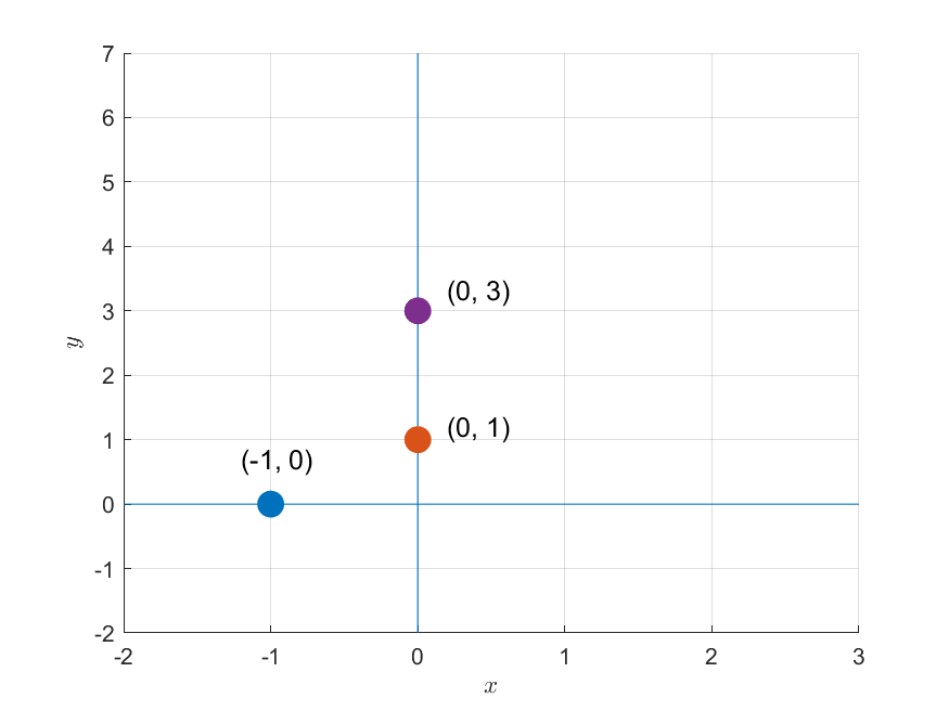
Figure 1. Three given data points

If we assume that we obtained these three data points through a model such as $f(x) = mx+b$, we can construct a system of three equations as follows:

\[f(-1) = -m + b = 0\] \[f(0) = 0 + b = 1\] \[f(0) = 0 + b = 3\]

If we represent this using matrices and vectors, we get the following:

\[(Ax = b) \Rightarrow\begin{bmatrix}-1 && 1 \\ 0 && 1 \\ 0 && 1\end{bmatrix}\begin{bmatrix}m \\ b\end{bmatrix} = \begin{bmatrix}0\\1 \\ 3 \end{bmatrix}\]

If we think about the problem of solving this matrix from a geometric perspective, it is equivalent to finding a line that passes through all three data points as shown in Figure 1.

No matter how we place a line on a two-dimensional plane, we cannot find a line that passes through all three points at the same time.

In other words, this problem cannot be solved because there is no solution.

Viewing systems of linear equations from a linear algebraic perspective

From the perspective of linear algebra, solving a system of linear equations can be thought of as solving the following matrix equation:

\[A\vec{x} = \vec{b}\]

Here, expressing both the vector and matrix as column vectors, and dividing the two elements of $\vec{x}$, we have:

\[\Rightarrow \begin{bmatrix} | & | \\ \vec{a}_1 & \vec{a}_2 \\ | & | \end{bmatrix}\begin{bmatrix}x_1 \\ x_2\end{bmatrix} = \begin{bmatrix}\text{ } | \text{ } \\ \text{ } \vec{b} \text{ }\\\text{ } | \text{ }\end{bmatrix}\]

Then, we can think of the above equation as follows:

\[\Rightarrow x_1\begin{bmatrix} | \\ \vec{a}_1 \\ | \end{bmatrix} + x_2\begin{bmatrix} | \\ \vec{a}_2 \\ | \end{bmatrix} = \begin{bmatrix}\text{ } | \text{ } \\ \text{ } \vec{b} \text{ }\\\text{ } | \text{ }\end{bmatrix}\]

In other words, it is like answering the question of how to combine the column vectors $\vec{a}_1$ and $\vec{a}_2$ to obtain $\vec{b}$ by providing the appropriate combination ratios of $x_1$ and $x_2$.

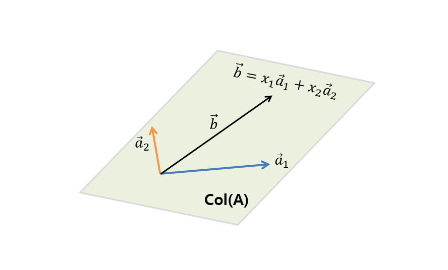
Figure 2. To find $\vec{b}$, which is included in the column space $col(A)$ of A, consisting of the column vectors ($\vec{a}_1$, $\vec{a}_2$) that make up A's column, how much should we combine $\vec{a}_1$ and $\vec{a}_2$?

However, to obtain $\vec{b}$ by combining $\vec{a}_1$ and $\vec{a}_2$, $\vec{b}$ must be one of the cases that can be obtained by combining all possible cases of $\vec{a}_1$ and $\vec{a}_2$.

In other words, $\vec{b}$ must be included in the column space (span) of $\vec{a}_1$ and $\vec{a}_2$. This is the condition for finding a solution.

Finding the optimal solution

As the saying goes, “A bird in the hand is worth two in the bush.” If we cannot find an exact answer to a problem like the one in Figure 1, we should at least try to find something that comes as close to the correct answer as possible.

In other words, we can try to find a line that can best represent the trend of the three points.

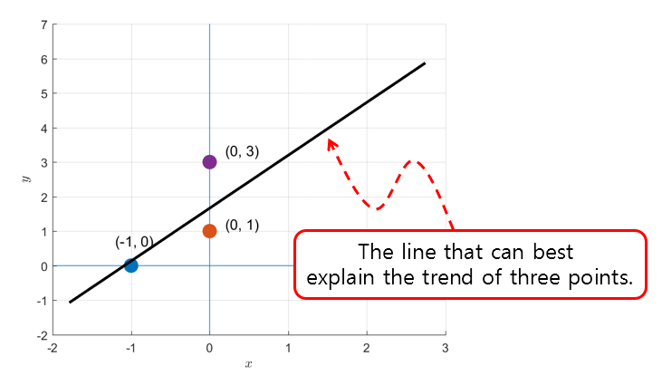
Figure 3. Let's try drawing a line that can best explain the trend of the three points.

Here, we can think of the process of finding the line that well represents the trend of the three points as finding the closest solution to the answer that exists in the column space of matrix $A$ when the solution ($\vec{b}$) does not exist in the column space.

In fact, if we draw $\vec{a}_1$, $\vec{a}_2$, the column space generated by these two vectors, and $\vec{b}$ directly in the problem of Figure 1 or Figure 3, it would look like the following.

Figure 4. The column space represented by the span of the two vectors $[-1, 0, 0]^T$ (blue) and $[1, 1, 1]^T$ (orange), and the vector $[0, 1, 3]^T$ (purple) that is not included in this column space.

If we abstract the contents of Figure 4 a little more, it would look like Figure 5 below.

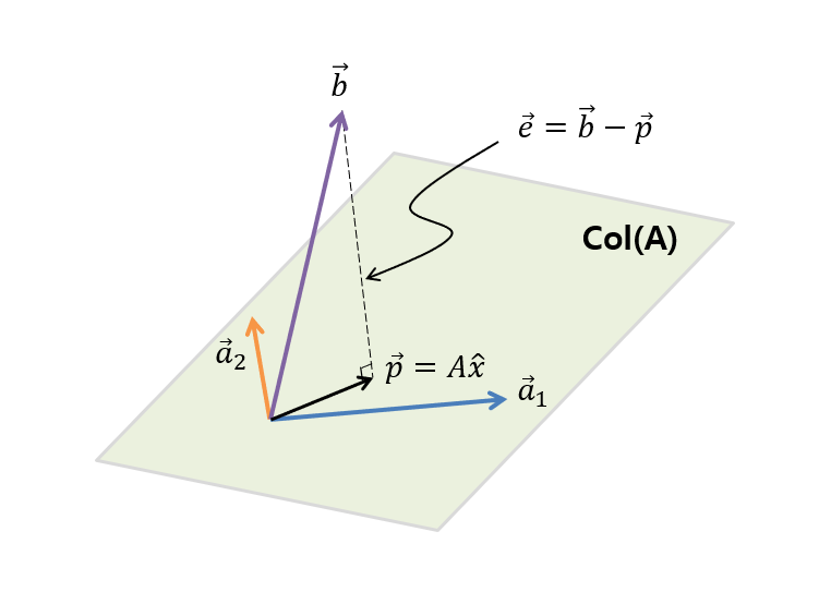
Figure 5. The column space $col(A)$ of A, which is made up of the columns of A's columns vectors ($\vec{a}_1$, $\vec{a}_2$), and the vector $\vec{b}$ that is not included in the column space.

As we can see in Figure 5, $\vec{b}$ is not included in the column space of $\vec{a}_1$ and $\vec{a}_2$. And as we can see in Figure 5, the optimal vector that is closest to $\vec{b}$ while also being obtained through a linear combination of $\vec{a}_1$ and $\vec{a}_2$, is the orthogonal projection of $\vec{b}$ onto the column space (col(A)), which we can calculate to find out how much we need to linearly combine $\vec{a}_1$ and $\vec{a}_2$ ($\hat{x}$).

If we denote the difference vector between the original solution vector $\vec{b}$ and the projection vector $\vec{p}$ as $\vec{e}$, then $\vec{e}$ is orthogonal to any vector in matrix $A$, and the following equation holds:

\[A\cdot\vec{e} = \begin{bmatrix} | & | \\ \vec{a}_1 & \vec{a}_2 \\ | & | \end{bmatrix}\cdot\vec{e} = 0\]

Here, ‘$\cdot$’ represents dot product.

In other words, by calculating the dot product, we have:

\[A^Te = A^T(\vec{b}-A\hat{x}) = 0\] \[\Rightarrow A^T\vec{b}-A^TA\hat{x} = 0\] \[\Rightarrow A^TA\hat{x} = A^T\vec{b}\] \[\therefore \hat{x}=(A^TA)^{-1}A^T\vec{b}\]

can be obtained.

Relationship with pseudoinverse

What have we done so far?

We have calculated $\hat{x}$ by multiplying an appropriate term to the left-hand side of the equation $Ax=b$.

In other words, we can see that the appropriate term found here can be denoted as $A^+$, and the fact that $A^+A = I$ is known.

In other words, we can see that the term we obtained, which is $(A^TA)^{-1}A^T$, is exactly the pseudoinverse we want to find.

Also, what does it mean that the result calculated in equation (9) is not equal to the right-hand side of equation (4)?

It means that the $\hat{x}$ obtained through the pseudoinverse is not the solution of the original equation (4), but it can be regarded as a combination of the column vectors of matrix $A$ to find the vector closest to $\vec{b}$ within the column space of matrix $A$.

Representation of Pseudo-Inverse using SVD

Any matrix $A\in\Bbb{R}^{m\times n}\text{ where } m\gt n$ can be written as a singular value decomposition (SVD) as follows.

\[A=U\Sigma V^T\]

Here, $U\in\Bbb{R}^{m\times m}$, $\Sigma\in\Bbb{R}^{m\times n}$, $V\in\Bbb{R}^{n\times n}$ are matrices of sizes, and $U$, $V$ are orthogonal matrices and $\Sigma$ is a diagonal matrix.

Here, $\Sigma$ is a matrix where the singular values $\lambda$ are located in the diagonal elements.

\[\Sigma = diag_{m,n}(\lambda_1, \cdots, \lambda_{min\lbrace m,n\rbrace})\]

Especially, the properties of orthogonal matrices are as follows.

\[UU^T = U^TU = I\] \[V^TV=V^TV = I\]

Also, the properties of diagonal matrices are as follows.

\[\Sigma^T = \Sigma\]

By taking the transpose of the SVD-decomposed $A$, it can be calculated as follows.

\[A^T = V\Sigma^T U^T=V\Sigma U^T\]

Therefore,

\[A^TA = V\Sigma U^T U \Sigma V^T\] \[=V\Sigma^2 V^T\]

Thus, to compute the inverse of $A^TA$,

\[(A^TA)^{-1} = (V\Sigma^2V^T)^{-1} = V(\Sigma^2)^{-1}V^T\]

From the above equation, the property of the orthogonal matrix $V$ that $V^{-1} = V^T$ is used.

Now, to compute the left pseudo-inverse in equation (1), it can be calculated as follows.

\[A^+ = (A^TA)^{-1}A^T = V(\Sigma^2)^{-1} V^TV\Sigma U^T\]

Here, $V^TV= I$, and $(\Sigma^2)^{-1}\Sigma = \Sigma^{-1}$, so the left pseudo-inverse using SVD is

\[\Rightarrow V\Sigma^{-1}U^T\]

Here, $\Sigma^{-1}$ is the following matrix.

\[\Sigma^{-1}=diag_{n,m}(\lambda_1^+, \cdots, \lambda^+_{min\lbrace m,n\rbrace})\]

where

\[\lambda^+=\begin{cases}\lambda^{-1} && \lambda \neq 0 \\ 0 && \lambda = 0 \end{cases}\]