Sampling from Probability Distributions

Samples from a uniform or normal distribution can be easily generated with just one line of code using a computer. For instance, in MATLAB, one can use the following code:

uniform_sample = rand(1,1)

normal_sample = randn(1,1)

However, how can we extract random samples from a probability density function (PDF) with an arbitrary formula?

Rejection Sampling

Suppose we have a PDF with an approximate formula that we know. For example, consider the following function $f(x)$:

This function $f(x)$ cannot be exactly called a probability density function because the area under this function from $-\infty$ to $\infty$ is not equal to 1, but rather equal to $\sqrt{5\pi}$.

However, when it is difficult to know the exact PDF, or when it is difficult to extract samples from the PDF with the given formula, a sampling method may be necessary.

We can name this probability distribution we want to extract samples from the “target distribution” and denote it as $f(x)$.

If we plot this target distribution, we can see that it has the following shape:

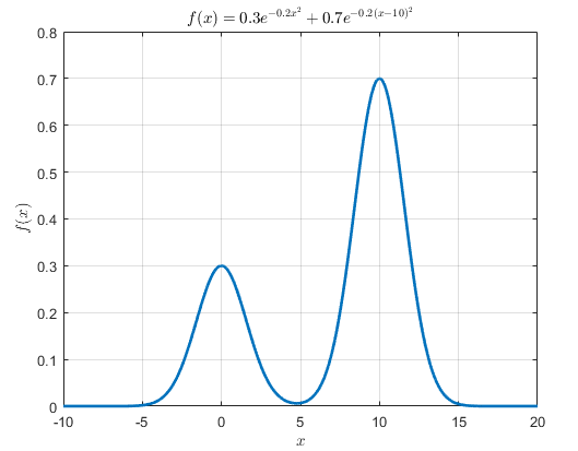
Figure 1. An arbitrary approximate PDF with a known formula

How can we extract samples from this approximate PDF? We can use a method called rejection sampling.

Proposal distribution

The first step in rejection sampling is to set the proposal distribution, also known as the proposal density.

Let’s denote the proposal distribution as $g(x)$ from now on.

We can generate the proposal distribution $g(x)$ using a distribution from which we can easily sample.

For example, we can use the uniform distribution as it is the simplest distribution to generate.

The textbook recommends setting the proposal distribution to be as similar as possible to the target distribution. However, using the uniform distribution is the easiest option.

Once we have decided on the proposal distribution, let’s draw the target and proposal distributions.

In this example, we set the domain of the uniform distribution we chose as the proposal distribution to include all possible target distributions within the range of $x$ as follows:

Then, our proposal distribution is as follows:

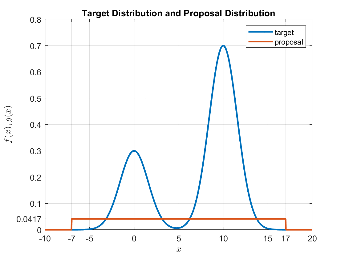
Figure 2. Target and proposal distributions.

Finally, we take a constant multiple ($M$) of the proposal distribution to also include the target distribution on the $y$-axis.

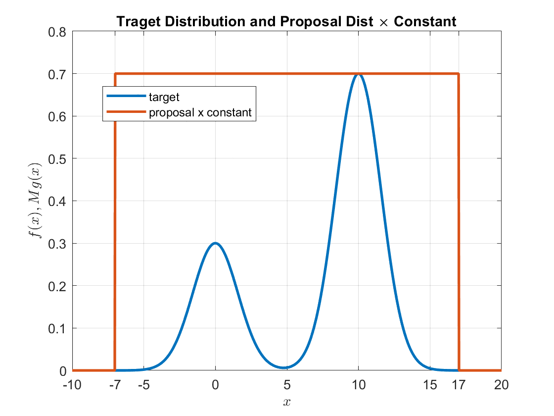
Figure 3. Target and proposal distributions multiplied by a constant to include the target distribution.

Sampling Process

Once we have chosen a proposal distribution and an appropriate constant, we can perform rejection sampling as follows:

The first step is to sample one point ($x_0$) from the proposal distribution $g(x)$.

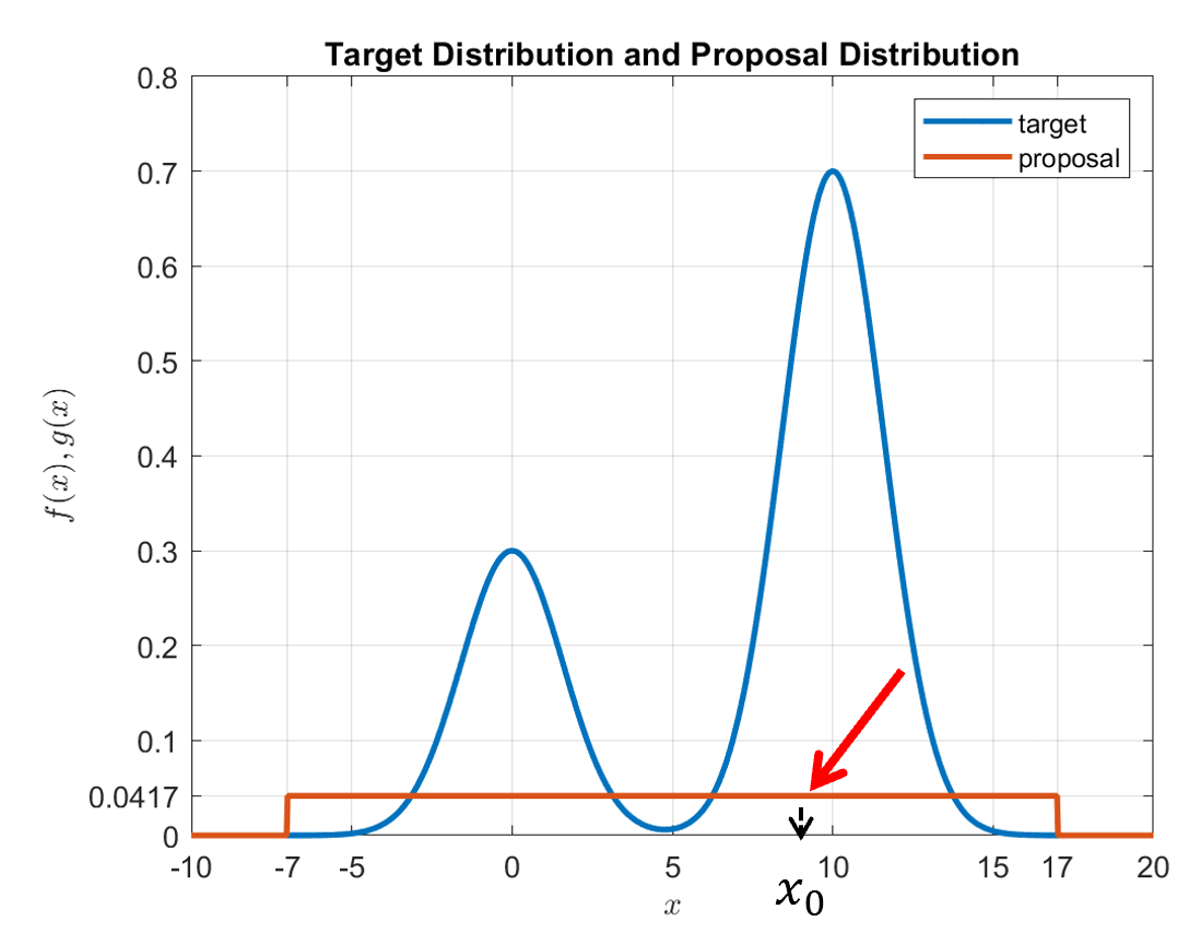
Figure 4. Sampling one point from the proposal distribution (in this case, a uniform distribution).

Next, we compare the likelihoods of the target distribution $f(x)$ and the scaled proposal distribution $Mg(x)$.

In other words, we compare the function values of $f(x_0)$ and $Mg(x_0)$ for the point $x_0$ sampled from the proposal distribution $g(x)$.

To perform the comparison, we divide the two function values and compare the resulting ratio.

That is, we use the following formula to perform the comparison:

If we think carefully about formula (4), we can see that if the target distribution is M times higher than the proposal distribution $g(x)$ at $x_0$, then the ratio will be close to 1, and if not, the ratio will be small.

Now we define the range of the ratio in terms of a uniform distribution with the following domain:

In other words, we can compare the value of formula (4) with a sample value from a uniform distribution with the domain mentioned above, as illustrated in the following figure:

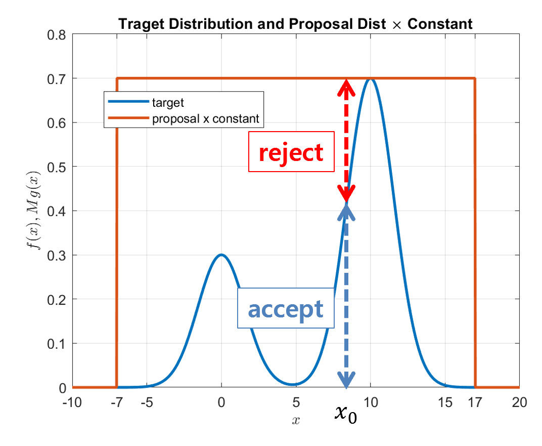
Figure 5. Comparing the likelihood ratio for a given $x_0$ to decide whether to accept or reject the sample.

As shown in Figure 5 above, when we compare the likelihood ratio with the output of a uniform distribution, the higher the target distribution $f(x)$ is relative to the proposal distribution $Mg(x)$, the higher the probability of accepting the sample.

It is worth noting that the output of the uniform distribution used for the comparison is a random value between 0 and 1.

To summarize, the algorithm can be summarized as follows:

Set $i = 1$ Repeat until $i=N$

1. Sample $x^{(i)} \sim q(x)$ and $u\sim U_{(0,1)}$.
2. If $u\lt \frac{f(x^{(i)})}{Mg(x^{(i)})}$, then accept $x^{(i)}$ and increment the counter $i$ by 1. Otherwise, reject.

Results of Rejection Sampling

A partial representation of the results of rejection sampling is as follows.

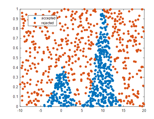
Figure 6. Accepted samples and rejected samples

And when the final obtained samples are plotted as a histogram along with the target distribution $f(x)$, which was originally intended to be obtained, it looks like the following.

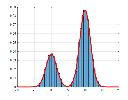
Figure 7. Target distribution $f(x)$ and the accepted samples plotted as a histogram.
(Note that the height of the $y$-axis is different from that of the other figures.)

The MATLAB code to obtain this result is as follows.

clear; close all; clc;

rng(1)
n = 500;
target = @(x) 0.3*exp(-0.2 * x.^2) + 0.7 * exp(-0.2 * (x - 10).^2);
xx = linspace(-10,20, 1000);

%% Sampling with the uniform distribution as the proposal distribution
% There is not much difference in performance, but the number of rejected samples is slightly different.

pseudo_dist2 = @(x) (x>=-10 * x<20) / 30;

figure;
plot(xx, target(xx));
hold on;
plot(xx, pseudo_dist2(xx)*21); % 21 indicates 30 * 0.7, where 30 is the range of x with output 1, and 0.7 is the maximum height of the target.

x_q = (rand(1, n) - 0.5) * 30 + 5; % uniform distribution between -10 and 20

crits = target(x_q) ./ (pseudo_dist2(x_q) * 21);
coins = rand(1, length(crits));

x_p_uniform = x_q(coins<crits);

figure; h = histogram(x_p_uniform,'BinWidth',0.5, 'Normalization','pdf');
hold on; plot(xx, target(xx)/max(target(xx))*max(h.Values))

Reference

• An introduction to MCMC for Maching Learning / C. Andrieu et al., Machine Learning, 50, 5-43, 2003