Signal Space

Prerequisites

To better understand this post, it is recommended that you have knowledge of the following:

Basic operations of vectors

Signals as Vectors

※ The contents of this section were taken from Linear operators and function spaces.

In a previous post, Basic operations of vectors (scalar multiplication, addition), which covered the basics of linear algebra, we considered vectors from three different perspectives.

These perspectives were that a vector is like an arrow, a list of numbers, and an element of a vector space.

Of these, we said that the definition of a vector as an element of a vector space is the most mathematical definition, and we emphasized that “defining vectors in this way highlights the fact that any concept with these characteristics can be treated as a vector and handled accordingly using techniques and concepts from linear algebra.”

In other words, if a concept has the properties of a vector, then techniques and concepts from linear algebra can be extended and applied to it.

To be more specific, in order for a mathematical object (such as a vector, matrix, signal, etc.) to be a vector, it must be closed under the following two operations:

Scalar multiplication of vectors
Vector addition

Is it too simple?

Just like how by paying a membership fee for Netflix’s membership gives you access to all videoss provided by Netflix, if it is confirmed that a mathematical object satisfies only these two laws, it becomes a member of the “vector” group.

And accordingly, it can receive the concepts and techniques that have been hard-earned in linear algebra.

Figure 1. Benefits that can be enjoyed by subscribing to Netflix (Source: Netflix)

Although not a rigorous proof, it is simple to see that a signal can be regarded as a vector.

Below are expressions for scaling a discrete signal and adding signals together.

\[(c\cdot x)[n] = c\cdot x[n] % Equation (1)\] \[(x+z)[n] = x[n]+z[n] % Equation (2)\]

In other words, if we multiply any signal $x[n]$ by an arbitrary constant $c$, $cx[n]$ is still a signal, and if we add any signals $x[n]$ and $z[n]$, $x[n]+z[n]$ is still a signal.

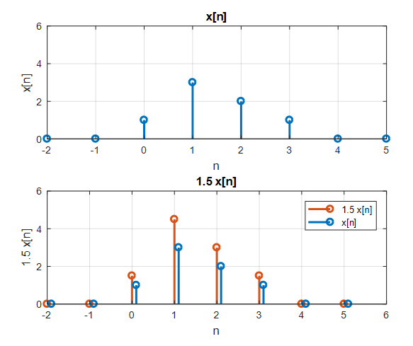
Figure 2. Scaling any arbitrary discrete signal still results in a discrete signal.

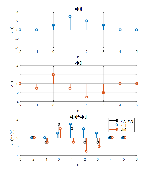
Figure 3. Adding any two arbitrary discrete signals still results in a discrete signal.

Not only discrete signals, but also continuous signals, when scaled or added together, remain continuous signals.

Figure 4. Sum of two continuous signals.
Image source: Function space, Wikipedia

Thus, as vectors are defined as elements of a vector space, signals can also be defined as elements of a vector space, and the vector space containing the signal is called the “signal space”.

We have seen that we can extend the concept of vectors to obtain the concept of signal spaces.

Now, the important point is which linear algebra concepts and techniques applicable to vectors can be applied to signals.

When we try to extend a concept, we must question even the most fundamental aspects. I think it is a wise start to question the concept of “coordinates” of a vector.

A signal is a point in signal space

When thinking about vectors, one of the first things that comes to mind is the definition of a vector as an arrow-like object. Many people tend to think of vectors as having “magnitude and direction”.

Although this definition of vectors only applies to Euclidean vectors and cannot be considered a general definition of vectors, it is a definition that provides a helpful way of visually understanding vectors.

(Once again, it is important to remember that what is required for something to be a vector is not just scalar multiplication and addition, but not necessarily having magnitude and direction. In order to have magnitude and direction, an inner product must be defined.)

In any case, let’s consider a point in 2-dimensional space. Let’s say the coordinates are (3,4).

When we say we are thinking of a vector with coordinates (3,4), we are simplifying an expression regarding how many base vectors in a 2-dimensional vector space we will combine.

The following figure shows a vector with coordinates (3,4) and two base vectors $\hat{i}$ and $\hat{j}$ in 2-dimensional vector space.

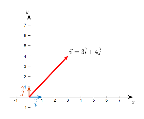
Figure 5. A vector with coordinates (3,4) and standard base vectors $\hat{i}$ and $\hat{j}$

And in the following figure, we can see that a vector with coordinates (3,4) can be composed by adding up 3 of one base vector and 4 of the other base vector.

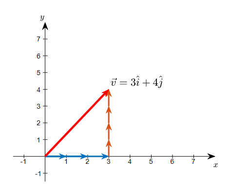
Figure 6. Saying that the coordinates are (3,4) means that the vector can be represented as a sum of three of one base vector and four of the other base vector.

So do we always have to use these standard base vectors? In fact, we can choose any two of the many 2-dimensional vectors to use as base vectors.

The following figure shows a new coordinate system created by rotating the coordinate system counterclockwise by 10 degrees. The base vectors in this new coordinate system are labeled as $\hat{i}{new}$ and $\hat{j}{new}$.

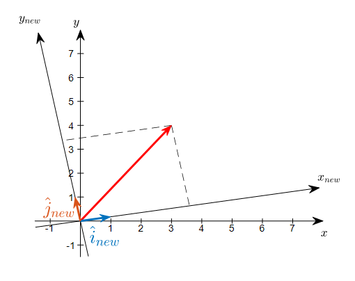
Figure 7. Can we represent the vector that was expressed as (3,4) in a coordinate system where a new set of base vectors is applied?

By using new basis vectors, the original vector can be expressed as coordinates (3.6, 3.4). This is equivalent to indicating how many basis vectors are included.

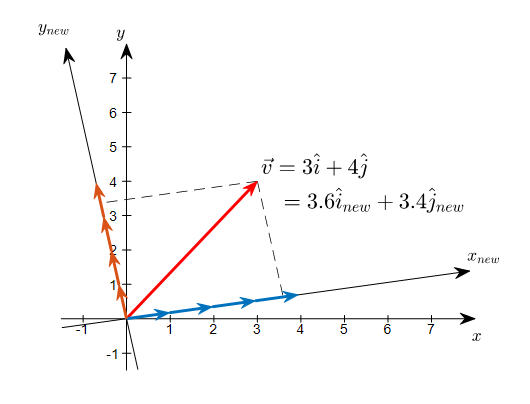
Figure 8. Using new basis vectors, the original vector can be represented using 3.6 and 3.4 of each basis vector, respectively.

In this way, a vector is like a point in vector space. However, the way to represent this vector depends on the basis.

In mathematical notation, any vector $\vec{v}$ can be written as a linear combination of basis vectors as follows:

\[\vec{v} = c_1 \hat{i} + c_2 \hat{j} = d_1 \hat{i}_{new} + d_2\hat{j}_{new}\]

Some bases can provide a simpler and more concise representation of the same vector compared to other bases.

In the previous example, $c_1$ and $c_2$ were simple values of 3 and 4, respectively, but $d_1$ and $d_2$ were slightly more complex values of 3.6 and 3.4.

Thus, selecting a good basis for representing the same vector is crucial.

Similarly, any arbitrary signal can be represented as a linear combination of basis signals in the signal space.

If an arbitrary signal $x[k], k = 1, 2, \cdots n$ is included in the signal space, the basis signals for the signal space can be denoted as $\lbrace \phi_i[k] | i = 1,2,\cdots, n\rbrace$. Then, any arbitrary signal $x[n]$ can be represented as a linear combination of basis signals as follows:

\[x[k] = \sum_{i=1}^{n}p_i \phi_i[k]\]

For continuous signals, any arbitrary signal $x(t)$ in the signal space that contains the basis signals can be represented as a linear combination of the basis signals $\lbrace \psi _i(t)\rbrace$ as follows:

\[x(t) = \sum_i q_i \psi_i(t)\]

Meanwhile, the number of basis vectors required to represent a vector can be calculated using the ‘dot product’ of vectors. That is, calculating $p_i$ and $q_i$ in the above equations is possible by defining the inner product of signals, similar to the inner product of vectors.

Inner product of vectors → Inner product of signals

In linear algebra, the inner product of vectors is defined as follows.

For any $n$-dimensional real vectors $\vec{a}$ and $\vec{b}$ as follows,

\[\vec{a} = \begin{bmatrix}a_1\\ a_2 \\ \vdots \\ a_n\end{bmatrix} % equation (6)\] \[\vec{b} = \begin{bmatrix}b_1\\ b_2 \\ \vdots \\ b_n\end{bmatrix} % equation (7)\] \[\text{dot}(\vec{a}, \vec{b})=a_1b_1 + a_2b_2 +\cdots + a_nb_n % equation (8)\]

If $\vec{a}$ and $\vec{b}$ were complex vectors, the inner product is defined as follows.

\[\text{dot}(\vec{a}, \vec{b})=a_1^*b_1 + a_2^*b_2 +\cdots + a_n^*b_n % equation (9)\]

Here, $*$ denotes the complex conjugate operation.

If we think about why complex vectors involve complex conjugate operations, it is to define the length of a complex vector through the inner product.

The size of a real vector $\vec{a}$ (usually L2-norm) is defined as follows.

\[\text{norm}_2(\vec{a}) = \sqrt{a_1^2 + a_2^2 + \cdots + a_n^2} % equation (10)\]

That is,

\[\text{norm}_2(\vec{a}) = \sqrt{\text{dot}(\vec{a}, \vec{a})}=\sqrt{a_1a_1+a_2a_2+\cdots+a_na_n} % equation (11)\]

If we extend this concept to complex vectors, then for a complex vector $\vec{a}$,

\[\text{norm}_2(\vec{a})=\sqrt{a_1^2+a_2^2 + \cdots a_n^2}=\sqrt{a_1^*a_1+a_2^*a_2+\cdots +a_n^*a_n}=\sqrt{\text{dot}(\vec{a},\vec{a})} % equation (12)\]

Therefore, the inner product operation of complex vectors must be defined as in equation (9).

Now let’s extend the method of equation (9) and define the inner product of signals.

Since signals can have complex values that do not end in the range of real signals, the definition of the inner product of complex vectors is extended as follows.

For discrete signals, the inner product of arbitrary complex discrete signals $x[k]$ and $z[k]$, $k = 1, 2, \cdots, n$ is defined as follows:

\[\langle x[k], z[k] \rangle \equiv \sum_{k=1}^n x[k]z^*[k]\]

Here, $z^*[k]$ is the complex conjugate of $z[k]$.

Moreover, for any complex continuous signals $x(t)$ and $z(t)$ defined on the interval $(a,b)$, the inner product $\langle f, g\rangle$ of the two signals is given by:

\[\langle x(t), z(t)\rangle \equiv \int_a^b x(t)z^*(t) dt % Equation (10)\]

where $z^*(t)$ is the complex conjugate of $z(t)$.

Eigenfunctions

To better understand eigenfunctions, it is recommended to have knowledge of the following:

Understanding eigenfunctions helps to explain why complex sinusoids are used to describe signals/systems in the field of signal processing.

In the previous discussion, we learned that a signal (i.e., a function) can be considered as a vector. Furthermore, since a signal is a vector, we can extend the terminologies and methods developed in linear algebra and apply them to signal processing.

One important topic in linear algebra is eigenvalues and eigenvectors, which can also be applied to signal processing.

To better understand the concept of eigenvectors, we need to understand the relationship between vectors and matrices.

A matrix can be considered as a function of vectors. Specifically, a matrix takes in a vector as input and outputs another vector.

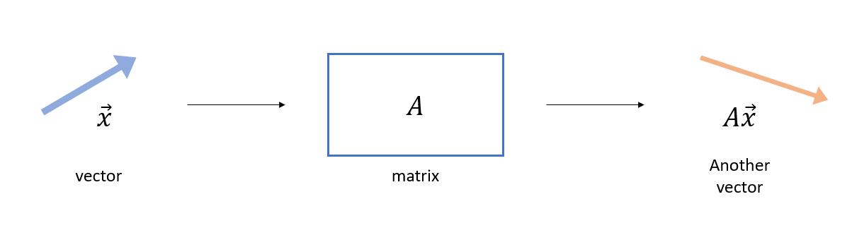
Figure 9. A matrix is a function that takes in a vector as input and outputs another vector.

In some cases, a matrix takes in a vector and outputs another vector whose direction is the same as the input vector, but whose magnitude is scaled by a constant.

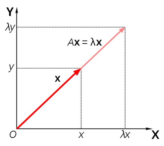
Figure 10. An input vector ($x$) and output vector ($Ax$) with the same direction but different magnitude.

In such cases, the unit vector pointing in the direction of vector $x$ is called the eigenvector of matrix $A$, and the amount of scaling is called the eigenvalue.

However, what about in signal systems that we study? If we consider signals as vectors, the system corresponds to a matrix.

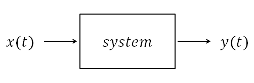
Figure 11. If signals correspond to vectors, the system corresponds to a matrix.

Then, is there a concept that corresponds to an eigenvector in the systems we deal with?

We usually call the concept that corresponds to eigenvectors in signals and systems eigenfunctions. (We usually do not call it an eigen signal.)

In most cases, in linear time-invariant (LTI) systems that we deal with, complex sinusoids become eigenfunctions.

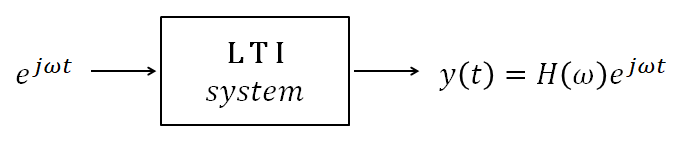
Figure 12. In LTI systems, complex sinusoids become eigenfunctions.

Looking a little more closely, if the input is $x(t) = e^{j\omega t}$ and the impulse response of the system is $h(t)$, then the output is

\[y(t) = \int_{-\infty}^{\infty}e^{j\omega (t-\tau)}h(\tau)d\tau\] \[=e^{j\omega t}\int_{-\infty}^{\infty}h(\tau)e^{-j\omega\tau}d\tau\]

Here, we define $H(\omega)$ as follows, which is called the Fourier transform of $h(t)$.

\[H(\omega) = \int_{-\infty}^{\infty}h(\tau)e^{-j\omega\tau}d\tau\]

The important thing is that if we rewrite the original equation,

\[y(t)=H(\omega)e^{j\omega t}\]

we can see that the original input function $e^{j\omega t}$ remains in the output function, and $H(\omega)$ is multiplied to it and then output.

It may seem natural for $e^{j\omega t}$ to appear so it may not seem special, but let’s try to input a cosine function this time.

A cosine function can also be written as follows using Euler’s formula.

\[x(t) = \cos(\omega t)=\frac{1}{2}(e^{j\omega t}+e^{-j\omega t})\]

If we call the system $\mathfrak L$, then the following equation holds because our system is a linear system:

\[y(t) = (\mathfrak{L}x)(t)=\frac{1}{2}\left(\mathfrak{L}(e^{j\omega t} + \mathfrak{L}(e^{-j\omega t})\right)\]

Using complex number notation here, if we express $H(\omega)$, we get:

\[H(\omega) = |H(\omega)|e^{j \angle H(\omega)}\] \[H(-\omega) = H^*(\omega) = |H(\omega)|e^{-j\angle H(\omega)}\]

Therefore, $y(t)$ can be rewritten as follows:

\[y(t) = \frac{1}{2}|H(\omega)|\left(e^{j(\omega t +\angle H(\omega))} + e^{-j(\omega t +\angle H(\omega))}\right)\] \[=|H(\omega)|\cos(\omega t + \angle H(\omega))\]

So when a cosine function is input, not only does its magnitude increase by $|H(\omega)|$ due to the system, but the phase also shifts by $\angle H(\omega)$, so it needs to be represented accordingly.

Therefore, when a cosine function is input, it is not an eigenfunction of a linear system since the input does not output the original input as it is.

What we can learn from this is that in the signal/system field, complex sinusoids are used to represent signals because when we use complex sinusoids to represent the input, we only need to describe the characteristics of the system (the Fourier transform of the impulse response) for the output, making the description of the output more concise.

References

PREVIOUSContinuous Time Convolution

NEXTContinuous Time Fourier Series