Try adjusting a, b, c, d to see the changes of phase plane.
Source: MIT Mathlets, https://mathlets.org/mathlets/vector-fields/

Prerequisites

To better understand the content about the phase plane, it is recommended to have knowledge about the following topics:

• Meaning of Euler’s number e
• Meaning of imaginary numbers
• Exponential function with a negative base
• Geometric interpretation of Euler’s formula
• Euler’s number e and homogeneous differential equations
• Meaning of eigenvalues and eigenvectors

Introduction to the Phase Plane

When interpreting first or second-order differential equations in mathematics, the use of the phase plane is critical in understanding the characteristics of the solutions of differential equations.

In the following second-order differential equation:

\[\begin{cases} \dfrac{dx}{dt} = f(x, y) \\\\ \dfrac{dy}{dt} = g(x, y)\end{cases} % Equation (1)\]

the phase plane can be drawn in a two-dimensional (or three-dimensional) real plane, where the slope of every point $(x, y)$ can be represented on the plane.

In other words, the slope at $(x, y)$ can be calculated as:

\[\frac{dy}{dx}=\frac{dy/dt}{dx/dt}\]

Therefore, we can compute the slope at all $(x, y)$ and draw it accordingly.

The most basic second-order differential equation is as follows:

\[\begin{cases} \dfrac{dx}{dt} = x \\\\ \dfrac{dy}{dt} = y\end{cases} % Equation (2)\]

The phase plane for Equation (2) is shown below.

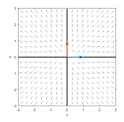
Figure 1. The phase plane for Equation (2). The arrows represent the eigenvectors of the unit matrix, and the thick black lines indicate the lines passing through the origin in the direction of the eigenvectors.

Another possible second-order differential equation is as follows:

\[\begin{cases} \dfrac{dx}{dt} = y \\\\ \dfrac{dy}{dt} = x\end{cases} % Equation (3)\]

The phase plane for Equation (3) is shown below.

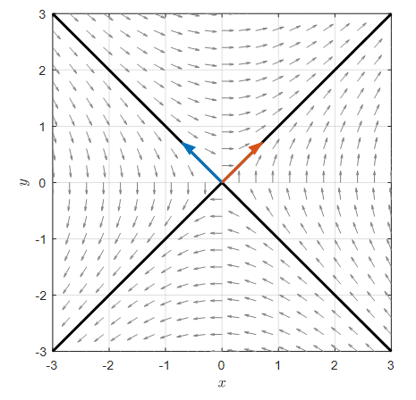
Figure 2. The phase plane for Equation (3). The arrows represent the eigenvectors of the unit matrix, and the thick black lines indicate the lines passing through the origin in the direction of the eigenvectors.

How to draw a phase plane by hand

How were the phase planes in Figures 1 and 2 obtained from equations (2) and (3)?

Of course, they were drawn with a computer, but we should understand the basic principles to better understand the phase plane.

Let’s assume we have a system of coupled differential equations like equation (1).

For an arbitrary point $(x,y)$, we can calculate $dx/dt$ and $dy/dt$ through equation (1).

By changing $dt$ to an appropriate size of $\Delta t$, we can calculate an appropriate size of $\Delta x$ and $\Delta y$.

For example, for equation (3), at the point (2, -1), $dx/dt = -1$ and $dy/dt = 2$.

Now we need to draw arrows. Arrows indicate the direction indicated by the derivative at the corresponding coordinate.

Both $dx/dt$ and $dy/dt$ are defined as limits of $\Delta x / \Delta t$ and $\Delta y / \Delta t$, respectively.

Therefore, let’s choose a $\Delta t$ value as a reference for drawing arrows. If this value is given, we can obtain $\Delta x$ and $\Delta y$.

For example, if we set $\Delta t = 0.1$, then $\Delta x = dx/dt * \Delta t = -0.1$ and $\Delta y = dy/dt * \Delta t = 0.2$. Therefore, at the point (2, -1), we can draw an arrow from (2, -1) to $(2+\Delta x, -1+ \Delta y)=(1.9, -0.8)$.

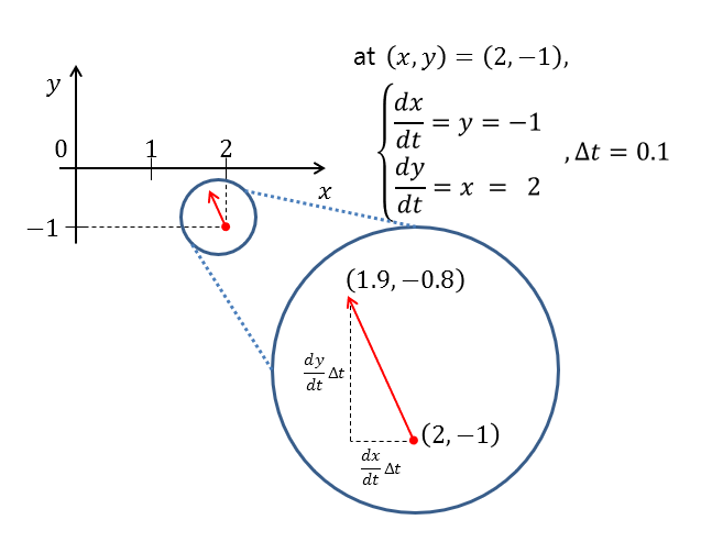
Figure 3. Result of drawing the vector at the point (2, -1) during the process of drawing the phase plane of equation (3)

By drawing arrows at every coordinate using this method, we can obtain a phase plane.

(Of course, drawing by hand is very time-consuming, so it is recommended to draw with a computer.)

What happens when you draw arrows continuously?

Let’s draw arrows continuously by increasing $\Delta t$ from 0.1 to 0.5.

Using the same method as described above, if we start from the point (2,-1) and set $\Delta t$ to 0.5, we can draw the trajectory of the position of $(x,y)$ coordinates with respect to time steps as shown in the figure below.

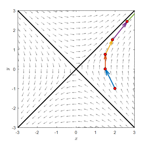
Figure 4. The path after 5 moves with $\Delta t = 0.5$ starting from the point (2,-1)

In Figure 4, as we multiply by $A$ starting from (2,-1), we can see that one black line approaches 0 and the other black line moves away from 0.

This result can be observed not only at point (2,-1) but also at any point on this plane.

In the figure below, we randomly selected four points and plotted the trajectory after five moves for each point with $\Delta t = 0.5$.

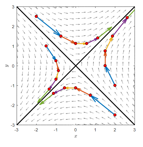
Figure 5. The path after 5 moves with $\Delta t = 0.5$ starting from four random points

For any of the four points, we can see that one black line approaches the origin and the other black line moves away from the origin.

So, what are these black lines and in what cases do the trajectories approach or move away from the origin?

Phase Plane and Matrices

What we can see through equations (1)~(3) is that the shape of the phase plane is determined by how we define $f(x,y)$ or $g(x,y)$ in equation (1).

One thing to consider here is that $f(x,y)$ and $g(x,y)$ are functions of $x$ and $y$, and one good way to combine them is to use matrices.

In other words, we can also view equation (1) as a system of differential equations using the following matrix.

\[\begin{bmatrix}dx/dt\\dy/dt \end{bmatrix} = \begin{bmatrix}a & b \\ c & d \end{bmatrix} \begin{bmatrix}x\\y\end{bmatrix}=A \begin{bmatrix}x\\y\end{bmatrix} % equation (4)\]

The Meaning of Eigenvectors in a System of Differential Equations

Looking at equation (4), we can see that a system of differential equations can be expressed using matrices. What information can we learn from the given matrix?

Equation (4) can also be written as follows.

\[\begin{bmatrix}dx/dt\\dy/dt \end{bmatrix} = \begin{bmatrix}a & b \\ c & d \end{bmatrix} \begin{bmatrix}x\\y\end{bmatrix}= \begin{bmatrix}a & b \\ c & d \end{bmatrix} \begin{bmatrix}1 & 0 \\ 0 & 1 \end{bmatrix} \begin{bmatrix}x\\y\end{bmatrix}% equation (5)\]

In other words, the slope of the phase plane that we are currently looking at, $dx/dt$ and $dy/dt$, can be transformed using the matrix

\[\begin{bmatrix}a & b \\ c & d\end{bmatrix}\]

from the original form

\[\begin{bmatrix}dx/dt\\dy/dt \end{bmatrix} = \begin{bmatrix}1 & 0 \\ 0 & 1 \end{bmatrix} \begin{bmatrix}x\\y\end{bmatrix}\]

as shown in equation (5).

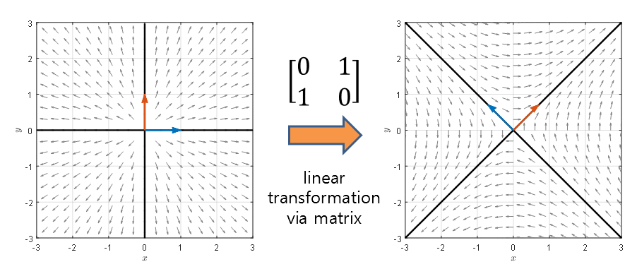
Figure 6. Linear Transformation by the Matrix $A$

In other words, the matrix $A$ can be thought of as a linear transformation applied to each vector on the phase plane on the left side of Figure 6. If you check the video, the following changes occur:

Figure 7. The function of the matrix as a linear transformation when considering the phase plane.

However, the arrows that were on the eigenvectors only changed in size, not in direction (they can go in the opposite direction). If we indicate the arrows on the eigenvectors with a different color, the result is as follows:

Figure 7. The direction of the arrows on the eigenvectors does not change during the linear transformation. (They can go in the opposite direction)

So why doesn’t the transformation by matrix $A$ affect the vectors represented in red?

Because the transformation applied by matrix $A$ moves along the eigenvector direction by a constant multiple on the eigenvector plane.

Furthermore, since the phase plane only represents the direction of the vector, not its magnitude, the red vectors do not show any change in direction. (However, if the eigenvalue is negative, it can move in the opposite direction.)

In other words, if we consider the definition of an eigenvector, if the vector before the transformation on the phase plane is a vector whose direction matches the eigenvector of matrix $A$, then only the magnitude changes, not the direction.

Therefore, the eigenvectors act as a new axis of transformation on the phase plane through matrix $A$.

In other words, when the matrix $A$ is as follows:

\[A=\begin{bmatrix}0 & 1 \\ 1 & 0 \end{bmatrix} % Equation (8)\]

The eigenvectors are as follows:

\[v_1 = \frac{1}{\sqrt{2}}\begin{bmatrix}-1\\1 \end{bmatrix}\] \[v_2 = \frac{1}{\sqrt{2}}\begin{bmatrix}1 \\1 \end{bmatrix}\]

Therefore, the lines $y=-x$ in the direction of $v_1$ and $y=x$ in the direction of $v_2$ act as new axes on the phase plane.

The Meaning of Eigenvalues in Differential Equation Systems

After learning about eigenvectors, let’s think about the meaning of eigenvalues.

Let’s recall the movement of solution curves at each step when we set $\Delta t = 0.5$ starting from $(2, -1)$, which we saw in Figure 4.

First of all, we confirmed earlier that eigenvectors act as the “axis” of new changes. Then, let’s think about the coordinates of the new “axis” according to the changes in the solution curve.

In the following figure, the arrows in the phase plane are removed for visualization, and only the changes in the solution at each time step are shown.

In addition, we projected the eigenvector $v_1$ on the $y=-x$ line and the eigenvector $v_2$ on the $y=x$ line and calculated the distance from the origin.

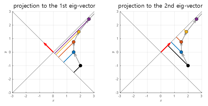
Figure 8. Let's project the coordinates of the solution at each time step onto the two eigenvectors and measure the distance from the origin.

If we mark the distance from the origin obtained in the figure above (i.e., the coordinate on the new axis), we can think about the following two methods:

The first method is to consider the coordinate value on the new axis as it is, and the second method is to think about how the coordinate value on the new axis changes according to the sequence.

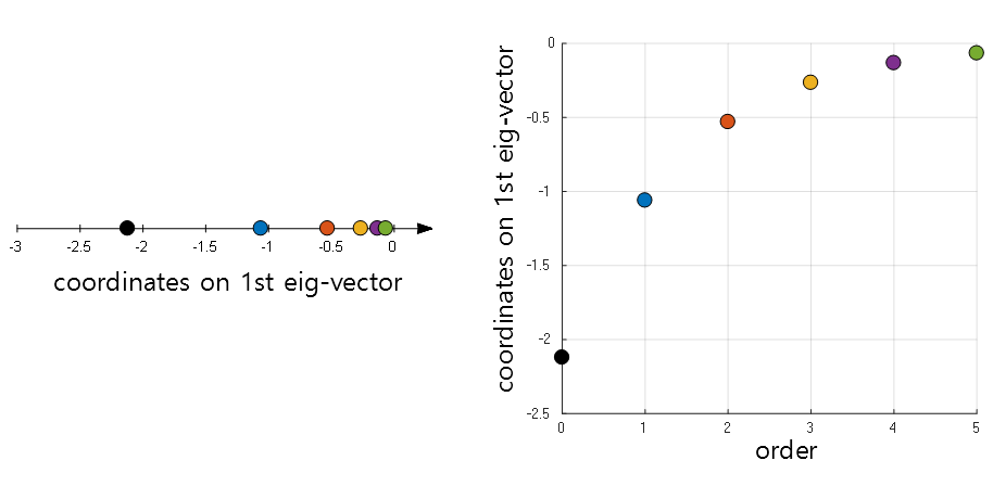
Figure 9. Changes in new coordinate values from the perspective of the first eigenvector

We can perform the same procedure on the second eigenvector.

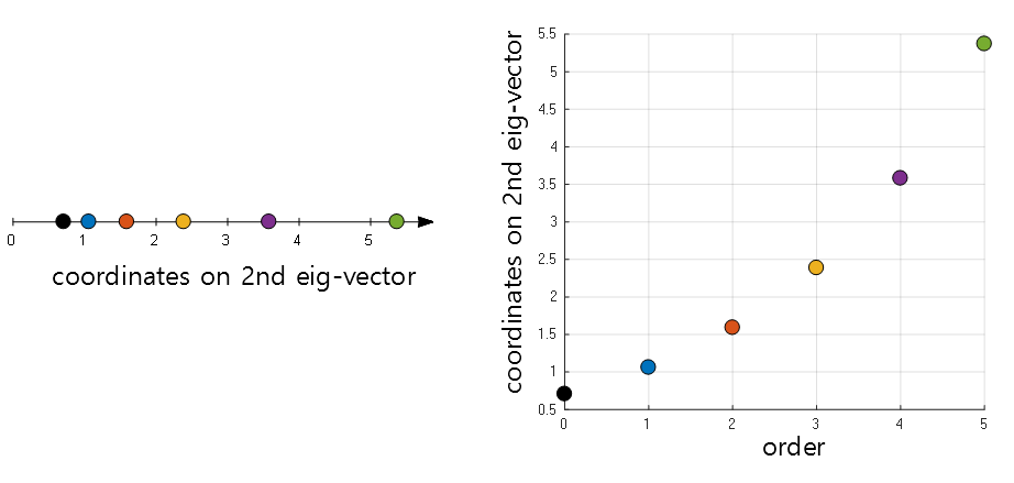
Figure 10. Changes in new coordinate values from the perspective of the second eigenvector

The eigenvalue of the first eigenvector was $-1$, and that of the second eigenvector was $1$. If we contrast this fact with the phenomena shown in Figure 9 and Figure 10, we can see that if the sign of the eigenvalue is negative, the coordinate value on the new eigenvector converges to 0 at each time step, and conversely, if the sign of the eigenvalue is positive, the coordinate value on the new eigenvector diverges to infinity at each time step.

In addition, looking at Figure 9 and Figure 10, we can see that the change in coordinate values for each type step shows an exponential change, as we saw in the ODE and Euler’s number e post, because it determines the position of the next solution curve on the basis of positive feedback. In other words, because the next value is determined based on the current value, it shows exponential change, and if $\Delta t$ becomes very small, it will grow continuously in the form of an exponential function with Euler’s number as the base.

Therefore, on each unique vector, the coordinates of the solution curve are determined through positive feedback, as in a first-order differential equation,

\[\frac{dx}{dt}=\lambda x\]

and the growth rate is determined by the magnitude of the eigenvalue.

Because, by definition of the eigenvalue, the growth on the eigenvector is only as large as the eigenvalue itself.

Therefore, the change in the coordinate values on each eigenvector can be written as

\[ce^{\lambda t}\]

where $c$ is a value determined by the initial value.

Solution of 2x2 First-order Linear Differential Equation

In conclusion, by considering the properties of eigenvalues and eigenvectors in a system of coupled homogeneous differential equations, we can think of a solution as follows:

\[\begin{bmatrix}x(t) \\y(t) \end{bmatrix}=c_1 v_1 \exp(\lambda_1 t) +c_2 v_2 \exp(\lambda_2 t)\]

In other words, the change occurs along the eigenvectors $v_1$ and $v_2$, but the coordinates on them change over time as $\exp(\lambda_1 t)$ and $\exp(\lambda_2 t)$.

$c_1$ and $c_2$ are values determined by the initial value.

Therefore, if the system of coupled differential equations in equation (4) has eigenvectors of $[-1, 1]^T$ and $[1, 1]^T$ and their corresponding eigenvalues are $-1$ and $1$, the solution will be as follows:

\[\begin{bmatrix}x(t) \\y(t) \end{bmatrix}=c_1 \frac{1}{\sqrt{2}}\begin{bmatrix}-1\\1 \end{bmatrix} \exp(-t) +c_2 \frac{1}{\sqrt{2}}\begin{bmatrix}1\\1 \end{bmatrix} \exp(t)\] \[=c_1 \begin{bmatrix}-1\\1 \end{bmatrix} e^{-t} +c_2 \begin{bmatrix}1\\1 \end{bmatrix} e^{t}\]

Moreover, if it passes through the point $(2, -1)$ at $t=0$, the solution curve is as follows:

\[\begin{bmatrix}2\\ -1 \end{bmatrix} = c_1\begin{bmatrix}-1 \\ 1\end{bmatrix}+c_2\begin{bmatrix}1 \\ 1\end{bmatrix}\] \[\therefore c_1 = -\frac{3}{2},\quad c_2 = \frac{1}{2}\] \[\therefore \begin{bmatrix}x(t) \\y(t) \end{bmatrix}=-\frac{3}{2}\begin{bmatrix}-1\\1 \end{bmatrix} e^{-t} +\frac{1}{2}\begin{bmatrix}1\\1 \end{bmatrix} e^{t}\]

This equation represents the equation of the curve expressed by the parameter $t$, and it can be represented as a graph as follows:

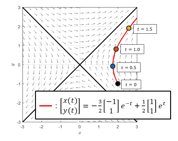
Figure 11. Graph of the curve represented by equation (17)

Furthermore, if we compare the coordinates on the eigenvector considered in Figures 9 and 10 with the actual coordinates of the solution, we get the following:

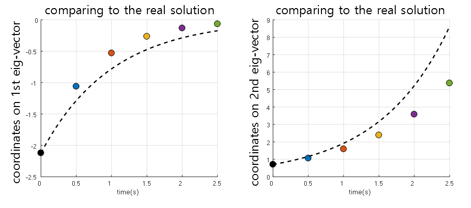
Figure 12. Comparison between the coordinates on the eigenvector considered with Euler's method and the actual solution.

The meaning of real numbers, complex numbers, and repeated eigenvalues

So far, we have seen that we can represent the changes of the solution curve over time on the phase plane, and that the motion occurs around the eigenvectors.

We also learned that the size and sign of the eigenvalues determine the rate of change of the solution curve over time, as well as the direction of whether it approaches or moves away from the origin.

Then, we can think of another thing here.

Let’s think about the fact that eigenvalues ​​are obtained by solving the characteristic equation as follows:

\[det(A-\lambda I)=0\]

If the eigenvalues were $\lambda =2, \text{ or } 3$ during this process, the characteristic equation would have been as follows:

\[(\lambda-2)(\lambda-3)=0\] \[\Rightarrow \lambda^2-5\lambda+6=0\]

What we can think about here is that this equation is a simple quadratic equation learned in middle school algebra.

Therefore, the solutions to the quadratic equation can be one of three cases: real, imaginary, or repeated roots.

Therefore, we can conclude the following:

Eigenvalues ​​can have real, complex, or repeated roots.

Cases with real eigenvalues

Cases with real eigenvalues ​​can be easily interpreted.

As we saw in equation (14), the eigenvalue is raised to the power of the natural constant $e$, and refer to the meaning of the natural constant e, the exponent above $e$ is proportional to the growth frequency and growth rate.

That is, if the eigenvalue is $\lambda = \alpha$, then if we raise it to the natural constant $e$ as in equation (14),

\[e^{\alpha t}\]

This is the amount of growth on the eigenvector. In other words, the amount that grows through positive feedback is determined as $t$ increases.

Therefore, in the case of having real roots, the solution curve shows changes such as approaching or moving away from the origin along the eigenvector, as shown in the figure below.

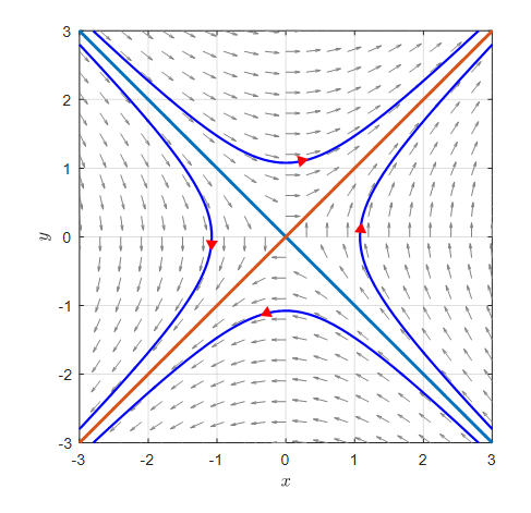
Figure 13. Example of the phase plane and some solution curves in the case of having real eigenvalues.

Case of having complex eigenvalues

In the case of having complex eigenvalues, some knowledge about imaginary numbers is required.

If you want to learn more about imaginary numbers, you can refer to the article about the existence and meaning of imaginary numbers. In short, multiplying a complex number by an imaginary number means a counterclockwise rotation of 90 degrees.

To summarize the key point, the involvement of imaginary numbers implies that there will be changes related to rotation.

However, as we saw in Equation (14), we raise the eigenvalues to the power of Euler’s number $e$.

So, what role do the eigenvalues play?

For example, let’s describe the eigenvalue in the following form of a complex number:

\[\lambda = \alpha + i\beta\]

Here, $\alpha$ and $\beta$ are both arbitrary real numbers, and $i=\sqrt{-1}$.

Then, if we raise $e$ to the power of $\alpha+i\beta$, we get:

\[e^{\lambda t}=e^{\alpha t + i\beta t}\]

And by the law of exponents,

\[\Rightarrow e^{\alpha t}e^{i\beta t}\]

We can say that $e^{\alpha t}$ means that the value continues to increase or decrease, as we saw in the case of having real eigenvalues.

However, what does $e^{i\beta t}$ mean?

This means a rotation on a circle with a radius of 1. If this concept is unfamiliar, you can refer to the article about the geometric meaning of Euler’s formula.

Generally, $e^{i\theta}$ represents a complex number that is located at the position obtained by rotating the number $1$ by $\theta$ radians in the complex plane.

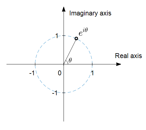
Figure 14. The position of the natural exponential function with imaginary exponent in the complex plane

Therefore, as time passes, $e^{\alpha t}$ increases in value, and since $e^{i\beta t}$ continues to rotate as time passes, the product of the two values, $e^{\alpha t}e^{i\beta t}$, takes the form of a circle whose radius increases as it rotates.

Figure 15. The change in position of the natural exponential function with complex exponent, $ re^{i\theta t}$, over time

Therefore, in the case of complex eigenvalues, if the real part is greater than 0, the solution curve has a continuously increasing radius.

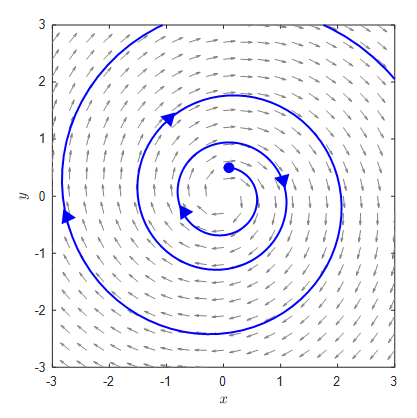
Figure 16. The solution curve in the case of complex eigenvalues with a real part greater than 0

On the other hand, in the case of complex eigenvalues, if the real part is less than 0, the solution curve has a continuously decreasing radius.

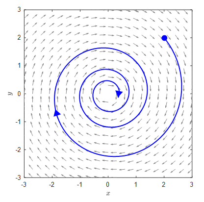
Figure 17. The solution curve in the case of complex eigenvalues with a real part less than 0

Cases of Repeated Eigenvalues

To consider the case of repeated eigenvalues, some thought is required.

First of all, having repeated eigenvalues means that these eigenvalues are always real numbers.

This is because the fact that the discriminant is 0, which determines the solution to the characteristic equation, ultimately indicates that the repeated root is always a real number.

In the case of having repeated eigenvalues, the solution can vary depending on whether the eigenvectors are linearly independent or not.

1. Case of Independent Eigenvectors with Repeated Eigenvalues

Let’s consider the following case:

\[\begin{bmatrix}dx/dt \\ dy/dt \end{bmatrix}=\begin{bmatrix}\lambda & 0 \\ 0 & \lambda \end{bmatrix}\begin{bmatrix}x \\y\end{bmatrix}\]

In this case, although the eigenvalues are all $\lambda$, the eigenvectors are

\[v_1 =\begin{bmatrix}1\\0\end{bmatrix},v_2 =\begin{bmatrix}0\\1\end{bmatrix}\]

corresponding to the $x$- and $y$-axes, respectively. Therefore, the solution can be obtained as follows:

\[\begin{bmatrix}x(t)\\y(t)\end{bmatrix}=c_1\begin{bmatrix}1 \\0\end{bmatrix}e^{\lambda t}+c_2\begin{bmatrix}0\\1\end{bmatrix}e^{\lambda t}\] \[=\begin{bmatrix}c_1\\c_2\end{bmatrix}e^{\lambda t}\]

2. Case of Repeated Eigenvalues with Repeated Eigenvectors

※ If you do not understand the following content, you can skip it without any problem in understanding the subsequent content.

(To understand this more precisely, it is recommended to understand basis transformation and standard form.)

Let’s consider the following case:

\[\begin{bmatrix}dx/dt \\ dy/dt \end{bmatrix}=\begin{bmatrix}\lambda & 1 \\ 0 & \lambda \end{bmatrix}\begin{bmatrix}x \\y\end{bmatrix}=A\begin{bmatrix}x \\y\end{bmatrix}\]

In this case, the eigenvalues are $\lambda$, with two identical eigenvalues, and the eigenvector is:

\[v=\begin{bmatrix}1\\0\end{bmatrix}\]

and only one comes out.

If we first calculate the first solution, we can see that:

\[s_1(t)= e^{\lambda t}\begin{bmatrix}1 \\0\end{bmatrix}\]

However, we can consider the second solution as follows ¹.

\[s_2(t) = te^{\lambda t}\begin{bmatrix}1\\0\end{bmatrix}+e^{\lambda t}\begin{bmatrix}v_3 \\ v_4\end{bmatrix}\]

And the final solution is considered as a linear combination of $s_1(t)$ and $s_2(t)$ as follows:

\[\begin{bmatrix}x(t)\\y(t)\end{bmatrix}=c_1s_1(t)+c_2s_2(t)\]

Since $s_2(t)$ must also satisfy the original differential equation, if we substitute it, we get:

\[s_2'=As_2\] \[\Rightarrow e^{\lambda t}\begin{bmatrix}1\\0\end{bmatrix}+t\lambda e^{\lambda t}\begin{bmatrix}1\\0\end{bmatrix}+\lambda e^{\lambda t}\begin{bmatrix}v_3\\v_4\end{bmatrix}=A\left(te^{\lambda t}\begin{bmatrix}1\\0\end{bmatrix}+e^{\lambda t}\begin{bmatrix}v_3 \\ v_4\end{bmatrix}\right)\]

Therefore, if we group both sides by $te^{\lambda t}$ and $e^{\lambda t}$, we can see that:

\[\left(\lambda\begin{bmatrix}1\\0\end{bmatrix}\right)te^{\lambda t}+\left(\begin{bmatrix}1\\0\end{bmatrix}+\lambda\begin{bmatrix}v_3 \\v_4\end{bmatrix}\right)e^{\lambda t}=\left(A\begin{bmatrix}1\\0\end{bmatrix}\right)te^{\lambda t}+\left(A\begin{bmatrix}v_3 \\v_4\end{bmatrix}\right)e^{\lambda t}\]

Thus, we can see that the following must be satisfied.

\[\begin{cases} A\begin{bmatrix}1\\0\end{bmatrix} = \lambda\begin{bmatrix}1\\0\end{bmatrix} \\\\ A\begin{bmatrix}v_3\\v_4\end{bmatrix}=\begin{bmatrix}1\\0\end{bmatrix}+\lambda\begin{bmatrix}v_3\\v_4\end{bmatrix} \end{cases}\]

In the first equation in the expression, there is nothing much to consider since it satisfies the original eigenvalue and eigenvector. Regarding the second equation, we can rewrite it as follows:

\[\Rightarrow \left(A-\lambda I\right)\begin{bmatrix}v_3\\v_4\end{bmatrix}=\begin{bmatrix}1\\0\end{bmatrix}\] \[=\begin{bmatrix}0&1\\0&0\end{bmatrix}\begin{bmatrix}v_3\\v_4\end{bmatrix}=\begin{bmatrix}1\\0\end{bmatrix}\]

Looking closely, we can see that $v_3$ is a free variable and $v_4=1$. Therefore, if we choose $v_3=0$,

\[\Rightarrow \begin{bmatrix}v_3\\v_4\end{bmatrix}=\begin{bmatrix}0\\1\end{bmatrix}\]

Thus, $s_2(t)$ becomes:

\[s_2(t)=te^{\lambda t}\begin{bmatrix}1\\0\end{bmatrix}+e^{\lambda t}\begin{bmatrix}0 \\ 1\end{bmatrix}=\begin{bmatrix}t\\1\end{bmatrix}e^{\lambda t}\]

Therefore, we can consider the solution to the system we wanted to find as follows:

\[\begin{bmatrix}x(t)\\y(t)\end{bmatrix}=c_1\begin{bmatrix}1 \\0\end{bmatrix}e^{\lambda t}+c_2\begin{bmatrix}t\\1\end{bmatrix}e^{\lambda t}\]

Let’s draw a phase plane for the following system of coupled differential equations:

\[\begin{bmatrix}dx/dt \\ dy/dt \end{bmatrix}=\begin{bmatrix}-1 & 1 \\ 0 & -1 \end{bmatrix}\begin{bmatrix}x \\y\end{bmatrix}=A\begin{bmatrix}x \\y\end{bmatrix}\]

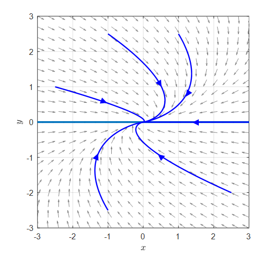
Figure 18. Phase plane of a system of coupled differential equations with duplicate eigenvalues and eigenvectors.