Plot of an approximation to the solution of dy/dx = x using the Euler method

Prerequisites

To better understand this content, it is recommended to know the following:

• Modeling phenomena with differential equations

Another perspective on differential equations

In the previous post on modeling phenomena with differential equations, we looked at how we can model phenomena using differential equations.

Most of the differential equations we used had a simple first-order form, which can be written as:

\[\frac{dy}{dx}=f(x,y) % Equation (1)\]

We can think of the left-hand side as the differential coefficient and the right-hand side as a polynomial, but we can also think of Equation (1) as a function value $f(x,y)$ defined by the $x,y$ coordinate system on the left-hand side and the differential coefficient on the right-hand side.

In other words, we can think of it as a form in which the slope is defined for all coordinates $(x,y)$.

Then, we can obtain the result of applying the differential coefficient to all coordinates in the form of a direction field or slope field.

In the example below, we have drawn a direction field for the following differential equation:

\[\frac{dy}{dx}=x % Equation (2)\]

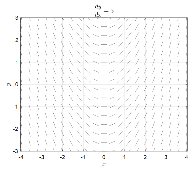
Figure 1. Direction field of dy/dx = x

What we can see in Figure 1 is that the differential coefficient or slope, called dy/dx, changes according to the x-coordinate values.

Although it is a formula obtained from a very simple differential equation, it can be a very good example to study direction fields.

So, what are the benefits of obtaining such direction fields when solving differential equations?

In the end, the ultimate result that can be obtained by studying differential equations is related to the solution of this equation, so the concept must be related to finding the solution.

Obtaining a solution using the Euler method

Let’s take a look at equation (2) used in Figure 1 again.

\[\frac{dy}{dx} = x \notag\]

The left-hand side in equation (2) is the rate of change. In other words, the differential equation in equation (2) tells us how the function changes moment by moment on the function according to the input value of x.

What exactly does “change” mean in a differential equation?

Change: Difference between the function value at the next point and the current point

Equation (2) may look difficult because it contains the differential coefficient dy/dx. Let’s go back to the original definition of the differential coefficient.

In other words, if we say y = f(x),

\[Equation (2) \Rightarrow \lim_{h\rightarrow 0}\frac{f(x+h)-f(x)}{h}=x % Equation (3)\]

we can express it as above.

If we think about this equation geometrically, we can think of it as shown in Figure 2 below.

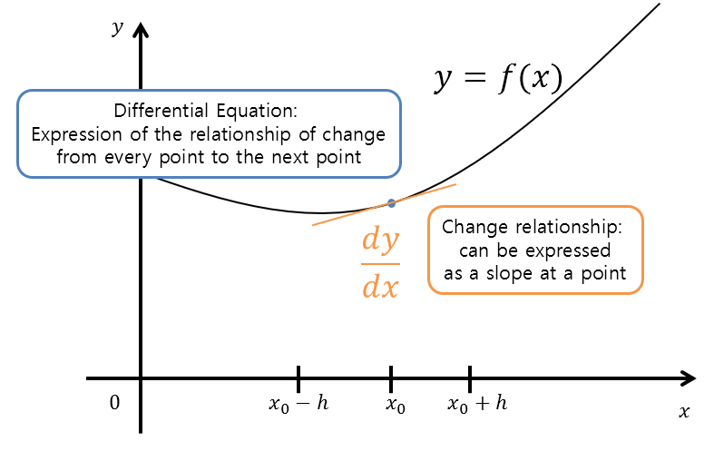
Figure 2. Geometric interpretation of differential equations

In other words, through the differential coefficient in differential equations, we can predict the function for the next domain value.

To think about the meaning of this, let’s try reducing the value of h from 1 little by little.

Case where $h=1$

\[Equation(3) \Rightarrow f(x+1)-f(x) = x % Equation (4)\] \[\Rightarrow f(x+1) = x + f(x) % Equation (5)\]

Therefore, what Equation (5) is saying is a kind of recurrence relation. If we set an initial value of $f(0)=0$, we can obtain $f(1), f(2), \cdots$ as follows.

\[f(1) = 0 + f(0) = 0 + 0 = 0 % Equation (6)\] \[f(2) = 1 + f(1) = 1+ 0 = 1 % Equation (7)\] \[f(3) = 2 + f(2) = 2 + 1 = 3 % Equation (8)\] \[f(4) = 3 + f(3) = 3 + 3 = 6 % Equation (9)\] \[\vdots\notag\]

Conversely, we can also obtain values like f(-1). Rewriting Equation (5) by moving x to the left-hand side, we have

\[f(x) = f(x+1) - x % Equation (10)\]

Therefore,

\[\Rightarrow f(x-1) = f(x) - (x-1) % Equation (11)\]

Thus,

\[f(-1) = f(0) - (-1) = 0 + 1 = 1 % Equation (12)\] \[f(-2) = f(-1) - (-2) = 1 + 2 = 3 % Equation (13)\] \[f(-3) = f(-2) - (-3) = 3 + 3 = 6 % Equation (14)\]

If we summarize some values in a table, we get the following.

And if we draw this on a graph, it will look like the following:

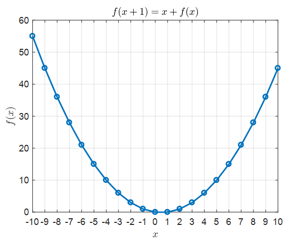
Figure 3. The solution of the recursion formula (5) plotted on a graph

Case where $h=0.5$

If $h=0.5$, then equation (3) will be changed as follows:

\[Equation(3)\Rightarrow \frac{f(x+0.5)-f(x)}{0.5} = x % Equation (15)\] \[\Rightarrow f(x+0.5) = 0.5x + f(x) % Equation (16)\]

Similar to equation (5), equation (16) can also be thought of as a recursion formula and by setting the initial condition $f(0)=0$, we can obtain values such as $f(0.5), f(1), f(1.5)$, etc.

Similarly, by adjusting equation (16) as follows, we can obtain values such as $f(-0.5), f(-1)$, etc.

\[\Rightarrow f(x-0.5)= f(x) - 0.5 (x-0.5) % Equation (17)\]

Some of the values are summarized in the table below.

And if we draw this on a graph, it will look like the following:

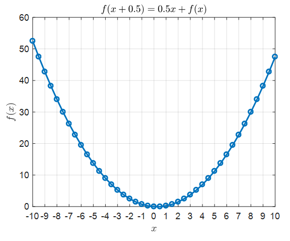
Figure 4. The solution of the recursion formula (16) plotted on a graph

Case where $h=0.1$

If we follow the same method for the case of $h=0.1$, we can obtain the following recurrence relation:

\[Equation(3) \Rightarrow \frac{f(x+0.1)-f(x)}{0.1} = x % Equation (18)\]

By using the same method, we can draw the solution of the recurrence relation on a graph as follows:

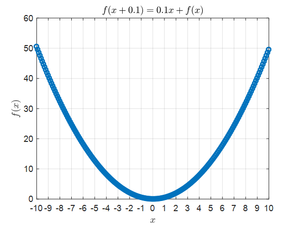
Figure 5. The solution of Equation (18) drawn on a graph.

Comparison of the True Solution of Equation (2) with Figures 2-4

However, Equation (2) can also be written as follows:

\[Equation(2) \Rightarrow f'(x)= x % Equation (19)\]

By integrating both sides of Equation (19) and applying the initial condition $f(0)=0$, we can obtain the following result:

\[f(x) = \frac{1}{2}x^2\]

That is, we can say that $f(x)=\frac{1}{2}x^2$ is the solution that satisfies Equation (2). Let’s compare this value with the values shown in Figures 2-4.

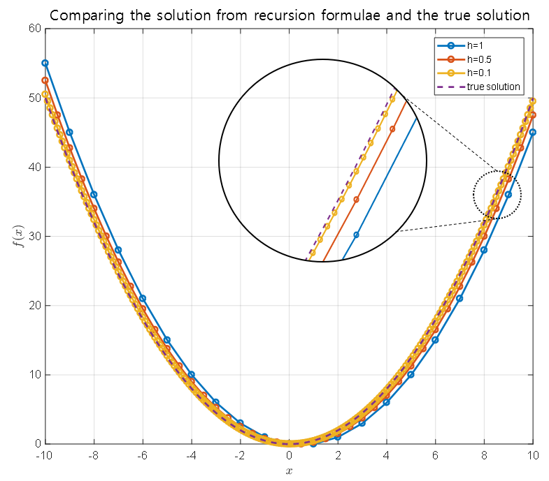
Figure 6. Comparison between the solution obtained from the recurrence relation shown in Figures 2-4 and the true solution of Equation (2).

By looking at Figure 6, we can see that the solution obtained from the recurrence relation and the true solution show similar results as $h$ becomes smaller.

In summary,

The method explained step by step in the previous content is the Euler method ¹.

Figure 7. Visual explanation of the Euler method
Figure source: Wikipedia: Euler method

The Euler method is a numerical method for solving differential equations, which indicates a few points to us:

1. Finding the solution of a differential equation means finding $f(x)$ that satisfies the differential equation.
2. The differential equation talks about the change in the function value, which tells us the difference in function value between the current point and the next point.
3. If we can determine only one starting point, we can obtain one solution curve according to the function value change rule described in the differential equation.
4. The smaller the gap between the current point and the next point, the closer the solution curve predicted by the Euler method will be to the true solution.

Initial Value Problem

The Euler method was a method of obtaining a solution based on the interpretation of primitive differential equations that explains the relationship between the function value and the change in the function.

Since we can know the relationship between the current function value and the surrounding function values, we can estimate the function value of the next domain value from one point.

Using this interpretation of primitive differential equations, the Euler method could estimate the function value and the surrounding function value from the given differential equation to find a solution.

Then, what is the ‘current function value’ mentioned so far?

Thinking about it, the ‘current function value’ mentioned here can be any point on the (x, y) plane. We can think of the solution of the differential equation regardless of the value we are looking at.

And the ‘relationship with the surrounding’ in the differential equation can be expressed as a slope. This is because the geometric meaning of the derivative is the slope.

In other words, using a differential equation, we can draw a slope at all (x, y) values.

If we draw the slope for the following differential equation used in the Euler method, we get the following for all points:

\[\frac{dy}{dx}=x\]

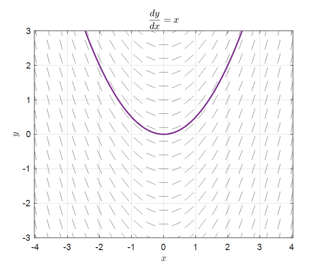
Figure 8. Slope field for dy/dx = x and one of its solutions, y = 1/2 * x^2

The red bars drawn in the figure represent the slope at each point (x, y).

Also, the purple line shaded in Figure 8 represents one of the solutions of equation (2), y = 1/2 * x^2.

What we need to consider here is that the purple line in Figure 8 is the line determined by the initial value y(0) = 0.

If the initial value is different, it will result in a different solution, as shown in the following figure.

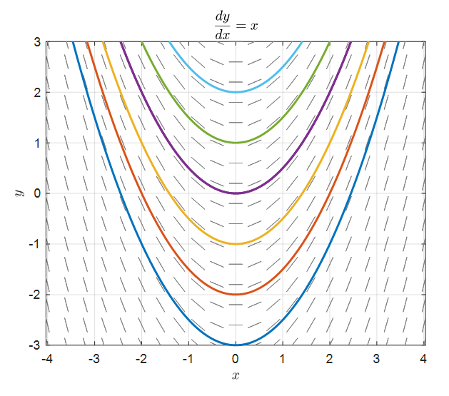
Figure 9. Solutions for dy/dx = x with various initial values

Checking the slope fields for other differential equations

In the previous post on modeling phenomena using differential equations, we looked at two first-order differential equation models.

They were Exponential growth and logistic growth models.

Let’s check the slope fields for each model.

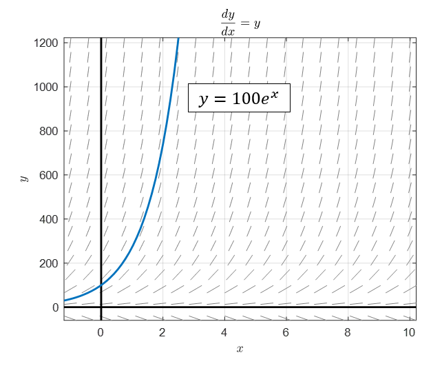
Figure 10. Slope field and solution with initial value of 100 for Exponential growth model

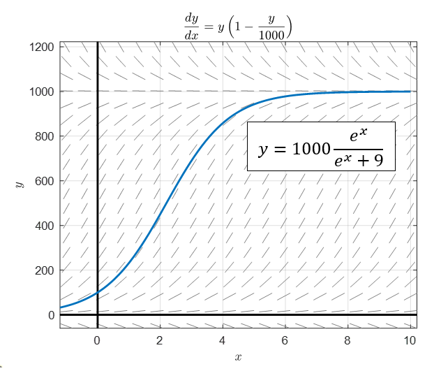
Figure 11. Slope field and solution with initial value of 100 for logistic growth model