The content of this post is largely borrowed from Thomas Judson’s The ordinary differential equations project.

A differential equation refers to an equation that contains a derivative.

In this case, the number of times the derivative is taken can be more than once.

The simplest form of a first-order differential equation is as follows:

\[\frac{dy}{dx}=f(x, y) % equation (1)\]

In this post, we will carefully explore how a differential equation like equation (1) can be derived.

Exponential Growth

Differential calculus is a mathematical description of “change.”

One example of a change that is easy to imagine is growth, and we will use the example of population growth to derive the form of a differential equation.

Population grows geometrically. To put it simply, we can think of it as follows:

Humans give birth to a portion of the population, and the population grows by some portion and decreases due to death.

Then, the growth of the population can be expressed as:

\[\text{Growth in Population}=\text{Births}-\text{Deaths} % equation (2)\]

We can see that we have not been considering time. This is an important point, and we should not overlook the fact that we need to think about growth in terms of “growth per unit time.”

If we do not specify whether the growth in equation (2) is for a million years or for one year, what does it mean?

Therefore, we can modify equation (2) as follows:

\[\text{Growth in Population during a certain period of time}=\text{Births per unit time}\cdot\text{certain period of time}-\text{Deaths per unit time}\cdot\text{certain period of time} % equation (3)\]

Equation (3) is a very verbose expression written in English. Let’s fix it and write it in mathematical notation.

The number of births per unit time will be proportional to the current population because only a portion of the current surviving population will give birth. The number of deaths per unit time can also be easily inferred to be proportional to the current population.

Let $P(t)$ denote the population at time $t$ and let $\Delta P$ denote the increase in population during a certain period of time. Let $k_\text{birth}$ and $k_\text{death}$ denote the rates of birth and death, respectively. Then we can write the following equation:

\[\text{Equation (3)} \Rightarrow \Delta P \approx k_\text{birth}P(t)\Delta t - k_\text{death}P(t)\Delta t %\text{Equation (4)}\]

If we slightly modify Equation (4) and let $k = k_\text{birth} - k_\text{death}$, we can write:

\[\Rightarrow \Delta P \approx kP(t)\Delta t %\text{Equation (5)}\]

Dividing both sides by $\Delta t$, we obtain:

\[\frac{\Delta P}{\Delta t} \approx k P(t) %\text{Equation (6)}\]

This means that the rate of change of population per unit time is proportional to the current population.

If we make $\Delta t$ very small in Equation (6), we can obtain a differential equation:

\[\Rightarrow \lim_{\Delta t \rightarrow 0}\frac{\Delta P}{\Delta t}=\frac{dP}{dt}%\text{Equation (7)}\]

Therefore,

\[\therefore \frac{dP}{dt}=kP %\text{Equation (8)}\]

We can see that Equation (8) has the same form as the differential equation shown in Equation (1).

The solution to the differential equation in equation (8) is given by

\[P(t) = Ce^{kt} % equation (9)\]

If we substitute equation (9) back into equation (8), we can see that

\[Cke^{kt} = kCe^{kt} % equation (10)\]

holds true.

If we know the initial population size, we can determine the value of $C$ in equation (9). For example, if the population size at $t=0$ is $P_0$, we can see that

\[\text{equation (9)}\Rightarrow P(t) = P_0e^{kt} % equation (11)\]

Logistic growth is a concept that is often mentioned in population studies. While populations can grow exponentially, there are limits to their growth. For example, South Korea is currently facing a declining birth rate, and if this trend continues, a future decline in population is inevitable.

Why can’t populations continue to grow indefinitely? This is because of the limits of resources. Just like bacteria in a petri dish cannot grow beyond the size of the dish, populations are constrained by the availability of resources.

Figure 1. Bacteria in a petri dish have limits on their population size and grow according to logistic growth.

Let’s modify equation (8) a bit to create a model where the growth rate slows down as it approaches the maximum growth potential.

We can modify equation (8) as follows:

\[Equation (8) \Rightarrow \frac{dP}{dt}=kP(1-\frac{P}{N}) % Equation (12)\]

In other words, we add a function $(1-P/N)$ to equation (8).

Here, $N$ is the maximum growth potential. Equation (12) tells us that the rate of change of population approaches 0 as $P$ approaches $N$. This is because as $P$ approaches $N$, $(1-P/N)$ approaches 0.

The solution for this type of model is known as:

\[P=\frac{N}{Ce^{-kt}+1} % Equation (13)\]

(It can be confirmed that equation (13) is the solution for equation (12).)

The graph of the solution with appropriate values for $N$, $C$, and $k$ is shown below.

In the graph below, we set $N$ to 1000, which means the maximum population capacity is 1000. As time passes, the population approaches 1000 and remains constant.

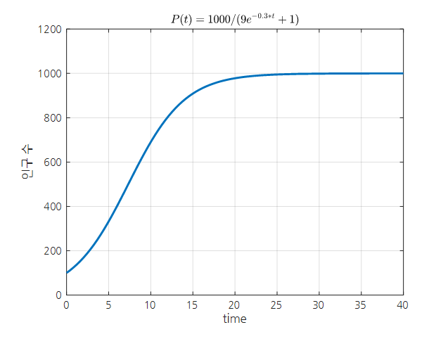
Figure 2. An example graph of logistic growth.

Phenomenon of movement in springs

Undamped spring-mass system

The formula for the movement of a spring, also known as Hooke’s law, is as follows:

\[F = -kx % Equation (14)\]

The negative sign indicates that the direction of the force acting on the spring is opposite to the direction in which the spring is stretched.

This equation is based on the observation of the following phenomenon, as shown in Figure 3:

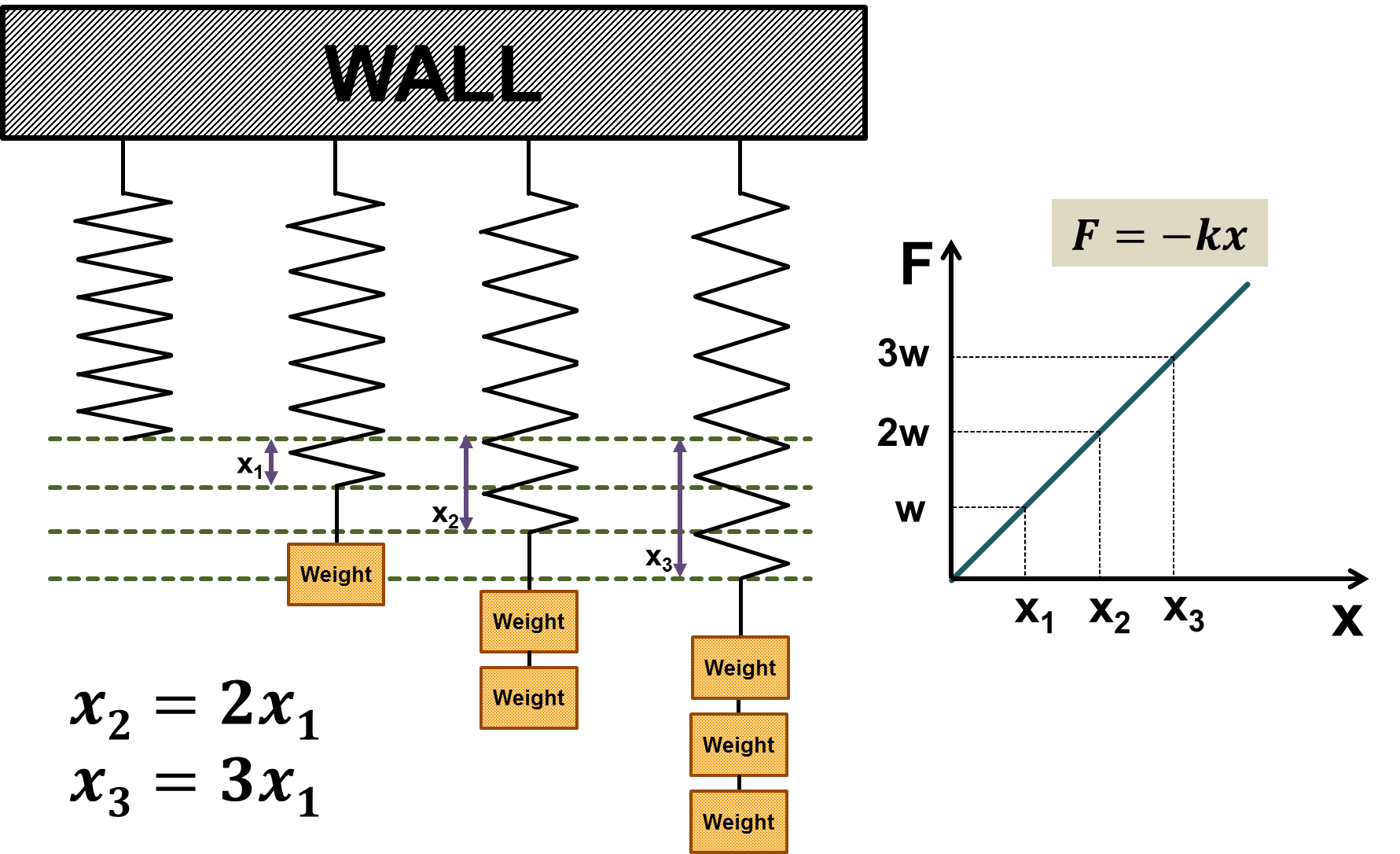
Figure 3. Experiment to derive Hooke's law
Source: Hooke's Law Wikipedia

As shown in Figure 3, it was experimentally discovered that the elastic force is proportional to the length of the stretched spring, which is explained by Equation (14).

Can we consider Equation (14) as a differential equation? Since force can be expressed as mass times acceleration, Equation (14) can also be written as follows:

\[m\frac{d^2x}{dt^2}=-kx % Equation (15)\]

Therefore, we can see that Hooke’s law is a second-order differential equation.

The solution to this differential equation is as follows:

\[x(t) = A\cos(t) + B \sin(t) % Equation (16)\]

If we assume that $m=1$, $k=1$, and the initial conditions are $x(0) = 0$ and $x’(0) = 1$, then Equation (16) becomes:

\[x(t) = \sin(t) % Equation (17)\]

The motion derived from Hooke’s law is usually referred to as the motion of an undamped spring-mass system and sometimes called harmonic motion.

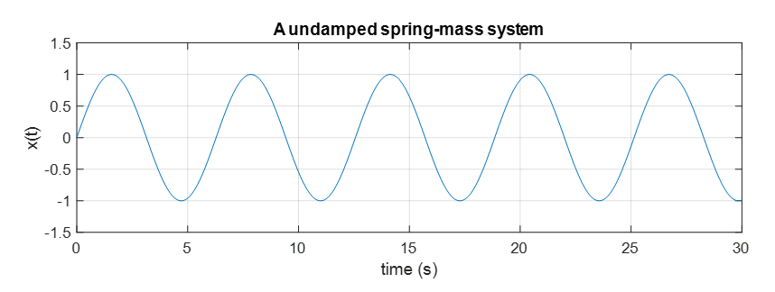
Figure 4. The motion of a spring assuming no damping is given by a sine function.

Damped spring-mass system

Before we look into damped motion, we need to think about what damping is.

Damping is a system that causes more force to be applied in the opposite direction as the object moves faster.

This method can be used to slow down the opening or closing of a door or to slow down the falling of an object.

The machine that provides damping motion is called a dashpot. You can see how a dashpot is used in the video below.

The damping motion provided by the dashpot is given in the opposite direction of the velocity, so it can be expressed as:

\[F = -b\frac{dx}{dt} \text{ where }b>0% Equation (18)\]

Therefore, if we add the equation for damping motion to the original equation (14), the equation is transformed as follows:

\[Equation(14) \Rightarrow F = -kx - b\frac{dx}{dt} % Equation (19)\]

or

\[m\frac{d^2x}{dt^2}=-kx-b\frac{dx}{dt} % Equation (20)\] \[\Rightarrow m\frac{d^2x}{dt^2}+b\frac{dx}{dt}+kx =0 % Equation (21)\]

We call such a model a simple damped harmonic oscillator.

We will learn how to solve differential equations such as Equation (21) later, but for now, let’s solve the problem assuming that the solution to this differential equation is of the following form.

\[x(t) = e^{rt} % Equation (22)\]

Substituting Equation (22) into Equation (21) yields

\[Equation (21) \Rightarrow mr^2e^{rt}+bre^{rt}+ke^{rt}=0 % Equation (23)\]

over-damped spring-mass system

Let’s assume that $m=1$, $b=3$, and $k=2$.

Then,

\[\Rightarrow r^2e^{rt}+3re^{rt}+2e^{rt}=0 % Equation (24)\] \[\Rightarrow e^{rt}(r^2+3r+2)=0 % Equation (25)\] \[\Rightarrow e^{rt}(r+1)(r+2) = 0 % Equation (26)\]

We can think that $e^{rt}$ is always positive, so $r=-1$ or $r=-2$.

Therefore, our solution should be of the following form.

\[x(t) = Ae^{-t}+Be^{-2t} % Equation (27)\]

If the initial value is given as follows:

\[x(0) = 0 % Equation (28)\] \[x'(0) = 1 % Equation (29)\]

We can calculate the values of $A$ and $B$ as follows.

\[x(0) = A+B = 0 % 식 (30)\] \[x'(t) = (-1)Ae^{-t}+(-2)Be^{-2t} % 식 (31)\] \[x'(0) = -1A-2B = 1 % 식 (32)\] \[\therefore A = 1, B = -1 % 식 (33)\]

Therefore, our solution is

\[Equation (27) \Rightarrow x(t) = e^{-t}-e^{-2t} % Equation (34)\]

as shown above.

If we draw a graph of Equation (34), we get:

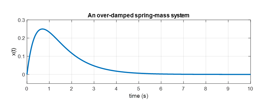
Figure 5. Solution curve of the over-damped spring-mass system when damping is greater than the spring force.

under-damped spring-mass system

Let’s say that instead of $k=2$, we have $k=38.25$. This means that the spring force is very strong and is designed to stretch easily with just a little force. In other words, damping acts as a small resistance to the movement of the spring.

If all other conditions are the same, the solution for this case can be found as:

\[\Rightarrow r^2e^{rt}+3re^{rt}+38.25e^{rt}=0 % Equation (35)\] \[\Rightarrow e^{rt}(r^2+3r+38.25) = 0\]

The solution for this case is

\[x(t) = e^{-\frac{3t}{2}}(A\cos(6t)+B\sin(6t))\]

If we insert the initial conditions from Equation (28) and Equation (29) back into the solution, we can find the values of $A$ and $B$:

\[x(0) = A = 0\] \[x'(t) = (-3/2)e^{\frac{-3t}{2}}(B\sin(6t))+e^{\frac{-3t}{2}}(6B\cos(6t))\] \[\Rightarrow x'(0) = 6B = 1\]

Therefore, we can find that the solution curve is as follows:

\[x(t) = \frac{1}{6}e^{-\frac{3t}{2}}\sin(6t)\]

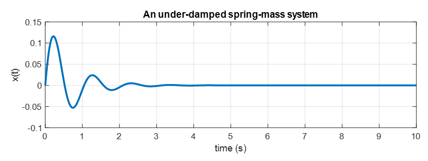
Figure 6. In case the force of spring is stronger than damping. The solution curve of under-damped spring-mass system

In conclusion

In this post, we modeled several phenomena using differential equations and found their solution curves. Differential equations can be considered a subject in which we learn how to find solutions to equations. It may be obvious, but when learning equations, we need to learn how to find their solutions. In the future, we will learn about:

• How to determine the process for finding solutions, which were skipped in the solution we found above.
• Whether these solution-finding methods always work.
• Whether the existence of a solution means that it is unique, even if the solution-finding method works.
• Whether all differential equations can be solved using one of these methods.