Prerequisites:

To better understand this post, it is recommended to be familiar with the following concepts:

• Continuous Time Fourier Series

The Idea of Fourier Transform:

The idea behind Fourier Transform is simple. For a periodic function $x(t)$ with a period of $T$, if we increase $T$ infinitely, it can be considered as an aperiodic function.

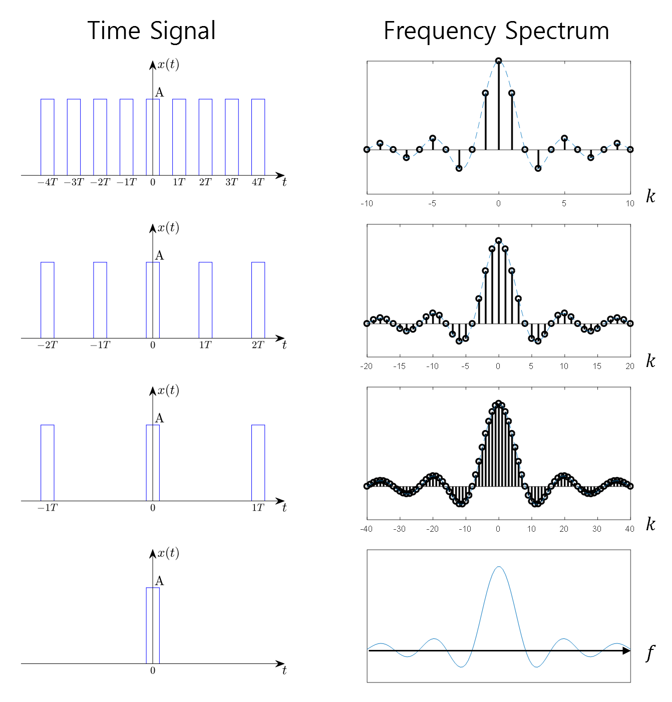
Figure 1. What happens when the period of a periodic function becomes infinitely large?

From the above figure, we can observe how the frequency spectrum changes as the period of a square pulse increases. In particular, we can see that the representation interval of the spectrum becomes narrower as the period increases.

As the period becomes infinitely large, the representation interval approaches zero, resulting in the frequency spectrum becoming a continuous signal.

The significance of Fourier Transform lies in the fact that any aperiodic function can be decomposed into sinusoidal functions, which implies its broad applicability.

In this post, we will explore the derivation process of Fourier Transform.

Derivation of Fourier Trnasform

A periodic function with a period of $T$ can be represented as follows:

\[x(t) = \sum_{k=-\infty}^{\infty}{c_k \exp\left(j \frac{2\pi k}{T}t\right)}\] where \[c_k = \frac{1}{T}\int_{0}^{T}{x(t)\exp\left(-j \frac{2\pi k}{T} t\right)dt}\]

In the process of transitioning from a Fourier series to a Fourier transform, what is needed is $T\rightarrow\infty$.

Since the function $x(t)$ in equation (2) is periodic, the following holds true:

\[c_k = \frac{1}{T}\int_{0}^{T}{x(t) \exp\left(-j \frac{2\pi k}{T}t\right)dt} = \frac{1}{T}\int_{-T/2}^{T/2}{x(t) \exp \left(-j \frac{2\pi k}{T}t\right)dt}\]

Substituting equation (3) into equation (1) and taking the limit of $T$ approaching infinity, we get:

\[\lim_{T\rightarrow \infty}x(t)= \lim_{T\rightarrow\infty} \sum_{k=-\infty}^{\infty}\left[\frac{1}{T}\int_{-T/2}^{T/2}{x(t) \exp\left(-j \frac{2\pi k}{T}t\right)dt}\right]\exp\left(j\frac{2\pi k}{T}t\right)\]

Let’s rearrange equation (4) slightly by moving $1/T$ to the far right of the right-hand side:

\[\lim_{T\rightarrow \infty}x(t)= \lim_{T\rightarrow\infty} \sum_{k=-\infty}^{\infty}\left[\int_{-T/2}^{T/2}{x(t) \exp\left(-j \frac{2\pi k}{T}t\right)dt}\right]\exp\left(j\frac{2\pi k}{T}t\right)\frac{1}{T}\]

Here, let’s keep in mind that some symbols in equation (5) can be replaced as follows, using the definition of definite integral:

• $1/T \rightarrow df$
• $k/T \rightarrow f$ ¹
• $T/2 \rightarrow \infty$
• $-T/2 \rightarrow -\infty$

For computational convenience, let’s first calculate the expression inside the square brackets ‘[ ]’ in equation (5):

\[\lim_{T\rightarrow\infty}\int_{-T/2}^{T/2}x(t) \exp\left(-j\frac{2\pi k}{T}t\right)dt = \int_{-\infty}^{\infty}x(t) \exp\left(-j2\pi f t\right)dt\]

The result of equation (6) can be interpreted as the Fourier transform of the signal $x(t)$.

In other words,

\[X(f) = \int_{-\infty}^{\infty}x(t) \exp\left(-j2\pi ft \right)dt\]

On the other hand, by substituting the result of equation (7) into equation (5), we can write it as follows:

\[\sum_{k=-\infty}^{\infty}\lim_{T\rightarrow\infty}X(f) \exp\left(j\frac{2\pi k}{T}t\right)\frac{1}{T}\]

Now, by the definition of definite integration, equation (8) can be written as follows:

\[\sum_{k=-\infty}^{\infty}\lim_{T\rightarrow\infty}X(f) \exp\left(j\frac{2\pi k}{T}t\right)\frac{1}{T}=\int_{-\infty}^{\infty}X(f) \exp\left(j2\pi f t\right)df\]

Through the above process, it is derived that any continuous-time function $x(t)$ can be Fourier transformed as follows:

\[x(t) = \int_{-\infty}^{\infty}X(f) \exp\left(j2\pi f t\right)df\] \[X(f) = \int_{-\infty}^{\infty}x(t) \exp\left(-j2\pi ft\right)dt\]

---

In addition, the convergence condition is necessary for the Fourier transformation. Since the magnitude of the complex exponential function $exp(-j2\pi ft)$ is 1, the convergence condition is as follows:

\[X(f) = \int_{-\infty}^{\infty}x(t) \exp\left(-j2\pi f t \right)dt \leq \int_{-\infty}^{\infty} x(t) dt \leq\int_{-\infty}^{\infty}|x(t)| dt < \infty\]

Furthermore, the signal should have a finite number of maxima and minima within any finite time interval, and the number of discontinuities of the signal within any finite time interval should also be finite. These conditions are necessary for the Fourier transformation.

Properties of Fourier Transform

The Fourier transform has several key properties.

Linearity

The Fourier transform is a linear transformation that satisfies the following property for any signals $x_1(t)$ and $x_2(t)$:

\[ax_1(t) + bx_2(t) \Longleftrightarrow a X_1(f) + b X_2(f)\]

Duality

Upon examining the formula of the Fourier transform in detail, we can observe that the formulas for $x(t)$ and $X(f)$ are almost identical, with the only difference being the sign of the exponent in the exponential function. If $x(t)\leftrightarrow X(f)$, the following property holds:

\[X(t) \Longleftrightarrow x(-f)\]

This is known as duality, and it allows us to easily obtain the Fourier transform of difficult signals using the duality property. For example, knowing that the Fourier transform of a rectangular pulse is a sinc function, we can deduce without additional calculations that the Fourier transform of a sinc function is a rectangular pulse.

Time Shift

Shifting a signal in the time domain by $t_0$ is equivalent to multiplying its Fourier transform by a complex exponential $\exp(-j2\pi ft_0)$ in the frequency domain:

\[x(t-t_0)\Longleftrightarrow X(f)\exp(-j2\pi ft_0)\]

This is because it introduces a phase delay of $t_0$ in the entire time signal.

Frequency Shift or Modulation

Multiplying a signal in the time domain by a complex exponential $\exp(j2\pi f_0 t)$ is equivalent to shifting the signal in the frequency domain by $f_0$:

\[\exp(j2\pi f_0 t)x(t) \Longleftrightarrow X(f-f_0)\]

By further applying this idea, we can consider the effect of multiplying the original signal by cosine and sine functions in the frequency domain:

\[\cos(2\pi f_0 t)x(t) = \frac{1}{2}\left(\exp(j2\pi f_0 t) + \exp(-j2\pi f_0 t)\right)x(t)\]

Thus,

\[\cos(2\pi f_0t) x(t)\Longleftrightarrow \frac{1}{2}\left(X(f-f_0) + X(f+f_0)\right)\]

Similarly,

\[\sin(2\pi f_0t) x(t)\Longleftrightarrow \frac{1}{j2}\left(X(f-f_0) - X(f+f_0)\right)\]

These frequency shifts or modulations are commonly used in AM (amplitude modulation) radio. AM radio transmits the original sound signal by modulating it onto a carrier signal. The carrier signal is a high-frequency signal that is advantageous for long-distance transmission, and this is achieved by performing amplitude modulation in this way.

Figure 2. AM, FM modulation

From the perspective of a receiving radio, demodulation is performed using the frequency of the carrier signal to restore the original audio signal (referred to as “signal” in Figure 2) for listening. Similarly, frequency modulation (FM) is another common modulation technique used in radio communication, where the frequency of the carrier signal is modulated according to the input signal.