What PCA tells you: If you need to reduce dimension of data by projecting it onto a vector,
which vector is the best to project in order to maintain the original structure of data?

※ This article follows column vector convention.

PCA: An Effective Method for Calculating Overall Scores

Let’s consider a scenario where 100 students took a Korean language test and an English language test.

Assuming that the English test was slightly more difficult, and the results were roughly as follows:

Korean Score	English Score
100	83
70	50
30	25
45	30
$\vdots$	$\vdots$
80	60

When visualizing the data with Korean scores on the x-axis and English scores on the y-axis, the distribution may look like the following (Figure 1).

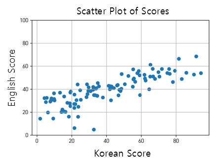
Figure 1. Distribution of example data

If we want to calculate an ‘overall score’ that combines Korean and English scores, what would be a good approach?

The first method that comes to mind is taking the average of the two scores. However, another approach could be to weigh the Korean and English scores in a 6:4 ratio, considering that the English test was relatively more difficult.

Mathematically, how would we express calculating the overall score by taking the average and weighing the scores in a 6:4 ratio?

For example, let’s consider a student, A, who scored 100 in Korean and 80 in English.

Calculating the average with a 5:5 ratio would be:

\[100 \times 0.5 + 80 \times 0.5\]

And calculating the overall score with a 6:4 ratio would be:

\[100\times 0.6 + 80 \times 0.4\]

If we explain using more mathematical terms, equation (1) is the dot product of the vector $(100, 80)$ and the vector $(0.5, 0.5)$, and equation (2) is the dot product of the vector $(100, 80)$ and the vector $(0.6, 0.4)$.

This can be represented graphically as follows:

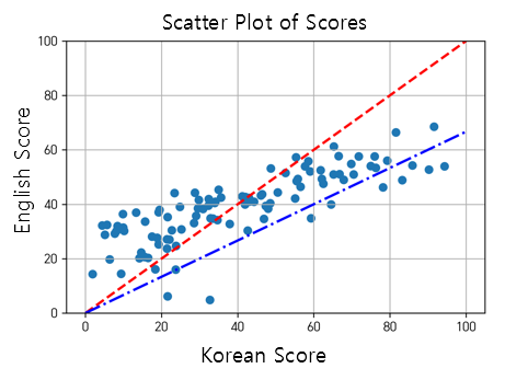
Figure 2. Distribution of example data and lines representing 5:5 and 6:4 ratios (in red and blue, respectively)

In other words, when obtaining a comprehensive score, the method of obtaining the score vector by dot product with a vector representing a specific ratio, such as 5:5 or 6:4, can be mathematically reduced to a problem of projecting the score vector onto a vector representing the ratio (in geometric terms, orthogonal projection).

Then, the key problem we need to consider is this:

• Which vector (or axis) to project the data vector onto in order to achieve the optimal result?

• As a secondary consideration, we can also think about:

• Wouldn’t it be better to find a vector that moves from the center of the data distribution as the pivot for the projection vector (or axis)?

The solution to this problem can be found from the covariance matrix, which is a mathematical representation of the ‘structure (or shape)’ of the data.

The Meaning of Covariance Matrix

The covariance matrix is a type of matrix that describes the structure of data, specifically showing how much variation between feature pairs (or in other words, how much they change together) is represented in the matrix.

Geometric Meaning of Covariance Matrix

Let’s now try to understand the covariance matrix geometrically. A matrix represents a linear transformation which has the ability to map one vector space linearly to another vector space.

In other words, we can view the data in the current distribution as “the original data distributed in the shape of a circle transformed by a linear transformation.” Let’s consider the distribution of data in the previous step of mapping by some matrix ¹ as shown below.

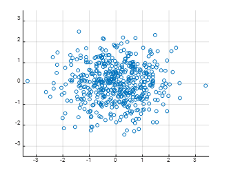
Figure 3. Random values distributed in a bivariate Gaussian distribution in a 2-dimensional vector space in a circular shape.

Let’s see what happens when we apply a matrix for linear transformation to the data in Figure 3 ¹. The linear transformation for the 2-dimensional vector space where the data is located is represented as shown in the applet below.

The covariance matrices of the resulting data obtained when each button is pressed are shown below.

Matrix 1: $\begin{bmatrix}3 & 2 \\2 & 4\end{bmatrix}$, Matrix 2: $\begin{bmatrix}3 & -2 \\-2 & 4\end{bmatrix}$, Matrix 3: $\begin{bmatrix}5 & 0 \\0 & 1\end{bmatrix}$, Matrix 4: $\begin{bmatrix}1 & 0 \\0 & 5\end{bmatrix}$

If we focus only on Matrix 1 out of the four matrices, the following can be observed from Matrix 1.

The element in the first row and first column of Matrix 1 represents the variance of the first feature. In other words, it indicates how much the data spreads along the x-axis.

The elements in the first row and second column, as well as the second row and first column, indicate how much the data spreads together along the x-axis and y-axis, respectively.

The element in the second row and second column indicates how much the data spreads along the y-axis.

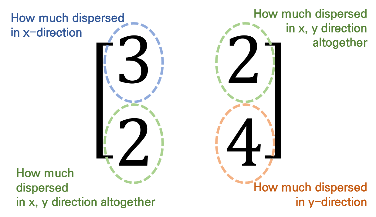
Figure 4. Meanings of each element in the covariance matrix, Matrix 1.

If we think carefully about the meaning of eigenvectors, they represent the directions of the principal axes along which the matrix acts on the vectors. Therefore, the eigenvectors of the covariance matrix indicate in which directions the data is dispersed.

Eigenvalues indicate how much the vector space is stretched along the direction of the corresponding eigenvectors². Thus, arranging the eigenvectors in descending order of their eigenvalues allows us to obtain the principal components in order of their importance. In Figure 5 below, we can see two eigenvectors and the magnitude of each vector represents its eigenvalue.

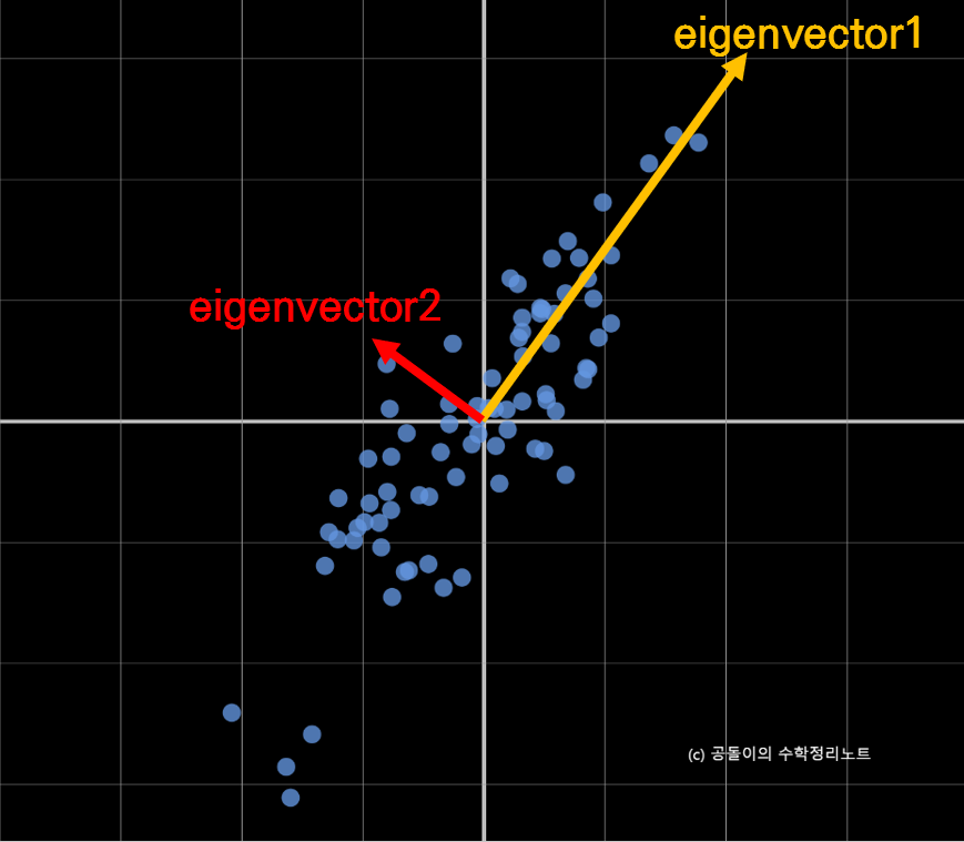
Figure 5. Eigenvectors of the covariance matrix, Matrix 1.

In other words, what was the question we were pondering? It is “Which vector should we use for inner product (or projection) of the data vector to obtain the optimal result?” This question can be answered by finding the eigenvalues and eigenvectors of the covariance matrix.

The Mathematical Meaning of Covariance Matrix

Let’s try to understand the covariance matrix mathematically. The covariance matrix is defined as a matrix that represents the covariance between two or more bivariate variables as a matrix. For example, let’s say we extract $d$ features from $n$ people, and represent the data as a matrix $X$ as shown in the figure below.

Assume that the mean value of each column (feature) of the matrix below is $0$. This assumption will help us to solve the ‘incidental problem’ explained earlier, which is finding a vector that moves the data distribution’s center along the pivot axis 1.

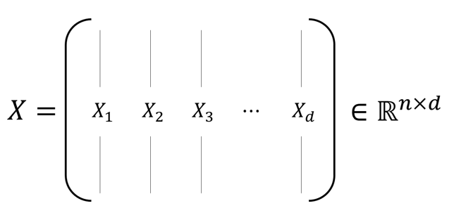
Figure 6. Data matrix X obtained by stacking d n-dimensional column vectors

Let’s consider an example of creating matrix $X$. Let’s put the height and weight of 5 people in matrix D as follows.

\[D = \begin{bmatrix} 170 & 70 \\ 150 & 45 \\ 160 & 55 \\ 180 & 60 \\ 170 & 80 \end{bmatrix}\]

Now, the matrix $X$ can be obtained from matrix $D$ by subtracting the mean of each column.

\[X = D - mean(D) = \begin{bmatrix} 170 & 70 \\ 150 & 45 \\ 160 & 55 \\ 180 & 60 \\ 172 & 80 \end{bmatrix} - \begin{bmatrix} 166 & 62 \\ 166 & 62 \\ 166 & 62 \\ 166 & 62 \\ 166 & 62 \end{bmatrix} = \begin{bmatrix} 4 & 8 \\ -16 & -17 \\ -6 & -7 \\ 14 & -2 \\ 6 & 18 \end{bmatrix}\]

Now, let’s try to obtain the covariance matrix using the data matrix $X$.

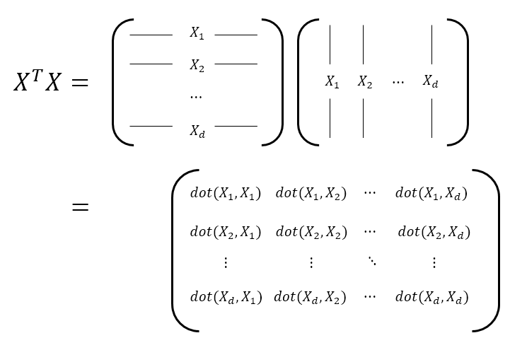
Figure 7. The process of calculating how similar the variations of each data feature are to each other in order to compute the covariance matrix.

Here, dot($\bullet$,$\bullet$) denotes the dot product operation between two vectors.

Now, what does $X^TX$ mean, as seen in Figure 7?

Looking at the last term in Figure 7, the element $(X^TX)_{ij}$ in the $i$th row and $j$th column of $X^TX$ indicates how similar the $i$th and $j$th features are among all the individuals, as obtained by taking the dot product of the values from all the individuals for the $i$th and $j$th features.

Let’s calculate $X^TX$ using the example we have been working on.

\[X^TX = \begin{bmatrix} 4 & -16 & -6 & 14 & 6 \\ 8 & -17 & -7 & -2 & 18 \end{bmatrix} \begin{bmatrix} 4 & 8 \\ -16 & -17 \\ -6 & -7 \\ 14 & -2 \\ 6 & 18 \end{bmatrix} = \begin{bmatrix} 540 &426 \\ 426 & 730 \end{bmatrix}\]

However, the issue with the $X^TX$ matrix is that the dot product values keep increasing as the number of samples $n$ gets larger. In other words, as more samples are accumulated, the resulting values become larger. To prevent this, we can divide the dot product values by $n$ to mitigate this issue. This leads us to consider the following matrix:

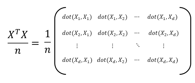
Figure 8. Calculation of the covariance matrix. Dividing the size of the matrix by the number of samples.

The matrix depicted in Figure 8 is called the covariance matrix. In other words, for the data matrix $X$, the covariance matrix $\Sigma$ is given by³

\[\Sigma = \frac{1}{n}X^TX\]

Let’s calculate the covariance matrix for the example data we have been working on.

\[\Sigma = \frac{1}{5}X^TX = \frac{1}{5} \begin{bmatrix} 540 &426 \\ 426 & 730 \end{bmatrix} = \begin{bmatrix} 108 & 85.2 \\ 85.2 & 146 \end{bmatrix}\]

Eigenvectors of Covariance Matrix and Maximum Variance

If the geometric explanation using eigenvectors and eigenvalues that was explained earlier was difficult to understand, the mathematical explanation in this part might be more helpful. In this part, we will explain why the variance of the data obtained by projecting it onto the eigenvectors⁴ is maximized.

Let’s say we project $d$-dimensional data onto a one-dimensional subspace through orthogonal projection. Consider an arbitrary unit vector $\vec{e}$ as the target of the projection. $\vec{e}$ is a $d \times 1$ dimensional vector. Then the projected data matrix $X\vec{e}$ can be written as $(X\vec{e})\vec{e}$, and its magnitude can be expressed as follows:

\[X\vec{e} \in \mathbb{R}^{n\times 1}\]

Therefore, the variance of the projected data onto $\vec{e}$ can be expressed as:

\[Var(X\vec{e}) = \frac{1}{n}\sum_{i=1}^{n}\left(X\vec{e} - E(X\vec{e})\right)^2\]

Assuming that the mean of each column of $X$ is 0, we can simplify the expression as follows:

\[Eq (9) = \frac{1}{n}\sum_{i=1}^{n}\left(X\vec{e} - E(X)\vec{e}\right)^2 =\frac{1}{n}\sum_{i=1}^{n}\left(X\vec{e}\right)^2\]

Thus,

\[Var(X\vec{e}) = \frac{1}{n}\left(X\vec{e}\right)^T\left(X\vec{e}\right)\] \[= \frac{1}{n}\vec{e}^TX^TX\vec{e} = \frac{1}{n}\vec{e}^T(X^TX)\vec{e}\] \[=\vec{e}^T\left(\frac{X^TX}{n}\right)\vec{e}\] \[=\vec{e}^T\Sigma\vec{e}\]

where $\Sigma$ is the covariance matrix.

Here, $\vec{e}$ was an arbitrary unit vector, and we want to determine how to choose $\vec{e}$ so that the variance of the projected data is maximized.

Let’s use the method of Lagrange multipliers. The objective function is

\[\vec{e}^T\Sigma\vec{e}\]

and the constraint is

\[\left|\vec{e}\right|^2=1\]

Thus, we can create the following auxiliary equation:

\[L = \vec{e}^T\Sigma\vec{e} - \lambda(\left|\vec{e}\right|^2-1)\]

Taking the partial derivative of $L$ with respect to $\vec{e}$, we get

\[\frac{\partial L}{\partial \vec{e}} = 2\Sigma\vec{e}-2\lambda\vec{e} = 0\]

So,

\[\Sigma\vec{e} = \lambda\vec{e}\]

This condition indicates that if we choose $\vec{e}$ that satisfies this equation, the objective function $\vec{e}^T\Sigma\vec{e}$ can be maximized.

Furthermore, from the result obtained by Lagrange multipliers, we can deduce that

\[Var(X\vec{e}) = \vec{e}^T\Sigma\vec{e} = \vec{e}^T\lambda\vec{e} = \lambda\vec{e}^T\vec{e} = \lambda\]

This shows that the variance of the projected data using the eigenvector is equal to the eigenvalue.

How many dimensions?

As we know, the main objective of PCA is to reduce the dimensionality of multidimensional data. But how far should we reduce the dimensionality of high-dimensional data?

Let’s say we reduce $d$-dimensional data to $m$ dimensions (where $m<d$). Since the data is $d$-dimensional, we can calculate a total of $d$ eigenvalues (assuming that the covariance matrix of the data is of full rank).

Let’s denote these eigenvalues as $\lambda_1, \lambda_2, \cdots, \lambda_d$ (where $\lambda_1 \geq \lambda_2 \geq \cdots, \geq \lambda_d$).

One logical approach is to reduce the dimensions up to a point where it explains, for example, 90% of the total data variance. In other words,

where we find an appropriate $m$ that satisfies the above equation, and reduce the dimensions up to $m$.

Another approach is to use a scree plot. This method can be somewhat subjective, where we plot a 2-dimensional graph with dimensions on the x-axis and corresponding eigenvalues on the y-axis. For example, the plot could look like this:

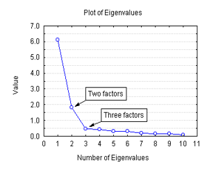
Figure 9: Example of a scree plot

From the plot, we can observe a sudden drop in eigenvalues starting from the third dimension. In this case, we can decide to reduce the dimensions up to 3 dimensions using the scree plot method. Scree plot is not only used in PCA but also in many other methods.