This post is a summary of a lecture by Professor Patrick H. Winston from MIT, which can be found at here.
1. Representing Hyperplanes using Vectors in n-dimensional Space
A hyperplane is defined as “a subspace of one dimension less than its ambient space” 1.
In other words, in an n-dimensional space, a hyperplane represents a subspace of dimension n-1. In the case of 3-dimensional space, a hyperplane is a 2-dimensional plane, while in 2-dimensional space, a hyperplane is a 1-dimensional line. To approach complex problems easily, let’s consider the equations for hyperplanes in 3-dimensional and 2-dimensional spaces, and generalize them for n-dimensional space.
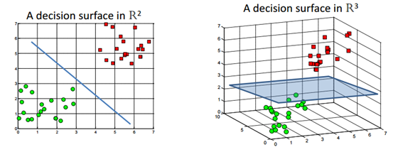
Figure 1. Decision surface. Source: Support Vector Machines without tears
The equation for a plane is as follows: for a normal vector $\vec{v}=(a,b,c)$, the equation of the plane with distance d from the origin is $ax+by+cz+d=0$. Now, let’s consider the case of 2 dimensions. If we apply this equation directly, the equation for a line with a distance d from the origin along a vector $\vec{w}=(a,b)$ would be $ax+by+d=0$.
If we slightly modify this equation, we can see that $y=-\frac{a}{b}x-\frac{d}{b}$. We can easily see that the slope of this linear function is perpendicular to the vector $\vec{w}$. Therefore, we can easily imagine hyperplanes in n-dimensional space using any normal vector and a real number.
Using this fact, we can define a hyperplane in n-dimensional real space as follows:
Definition 1. Hyperplane2
Let $a_1,a_2,\cdots,a_n$ be scalars not all equal to 0. Then set consisting of all vectors
\[X = \begin{bmatrix} x_1\\ x2\\ \vdots \\x_n \end{bmatrix}\in\Bbb{R}^n\]such that
\[a_1x_1 + a2_x2 + \cdots + a_nx_n = c\]for c a constant is a subspace of $R^n$ called a hyperplane.
2. Understanding Lagrange Multipliers
Lagrange multipliers are a mathematical technique used in optimization problems to find the maximum or minimum value of a function subject to constraints. The method of Lagrange multipliers involves creating an auxiliary equation using the objective function f(x, y) and the constraint g(x, y) = 0, introducing a new variable λ and solving for the values of x, y, and λ that satisfy the condition that the partial derivatives of the auxiliary equation with respect to all variables are equal to zero.
\[L(x, y, \lambda) = f(x,y) - \lambda g(x,y)\]The reason why this method can be used to solve optimization problems subject to constraints is that, at the point where the constraint is satisfied, the gradient of the objective function and the gradient of the constraint are parallel. By creating the auxiliary equation as described above, we can find the optimal values of the variables that satisfy both the objective function and the constraint. The figures below illustrate this concept.
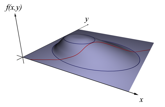
Figure 2. Explanation of Lagrange multipliers (1). Source: Wikipedia
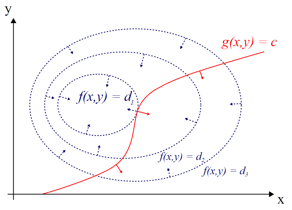
Figure 3. Explanation of Lagrange multipliers (2). Source: Wikipedia
In figures 2 and 3, the value of $f(x,y)$ can vary from $d_1$ to $d_3$, and suppose there is a constraint $g(x,y)=c$. What is the maximum value of $f(x,y)$ that satisfies the constraint? It is certainly $d_1$.
By closely observing Figure 3, we can see that the point where $f(x,y)$ and $g(x,y)=c$ intersect is the maximum value of $f(x,y)$ that satisfies the constraint. The condition for finding this point is that the slopes of the two curves are parallel. We can find the slope of a curve by taking its derivative, and in the case of multiple variables, we can use partial derivatives or gradients. Therefore, the condition for finding the point of intersection is as follows.
\[\nabla_{x, y}f = \lambda\nabla_{x, y}g\]where
\[\nabla_{x,y}f = \left(\frac{\partial f}{\partial x}, \frac{\partial f}{\partial y}\right)\]\(\nabla_{x,y}g = \left(\frac{\partial g}{\partial x}, \frac{\partial g}{\partial y}\right)\) In addition, in cases where there are multiple constraints, it may be possible to create the following:
\[L(x_1, \cdots, x_n, \lambda_1, \cdots, \lambda_M) = f(x_1,\cdots, x_n)-\sum_{k=1}^M{\lambda_kg_k(x_1,\cdots,x_n)}\]In other words, by finding the solution of the above equation, the optimization conditions can be found for cases where multiple constraints are imposed.
\[\nabla_{x_1, \cdots, x_n,\lambda_1,\cdots,\lambda_M}L(x_1, \cdots, x_n, \lambda_1,\cdots, \lambda_M) = 0 \Leftrightarrow \begin{cases}\nabla f(x)-\sum_{k=1}^{M}\lambda_kg_k(x)\\g_1(x) = \cdots = g_M(x) = 0\end{cases}\]3. Support Vector Machine
a. Decision Rule
The decision rule is a method for determining whether a new input $\vec{u}$ belongs to the class + or -. Assuming there is a decision boundary (hyperplane) and a normal vector $\vec{w}$ on a two-dimensional plane, we want to classify the input as + if it is above the dashed line in the middle, and as - if it is below. Therefore, we can set the decision rule as follows:
\[\vec{w}\cdot\vec{u} \geq c\]Here, c is an arbitrary constant. We can set the decision rule as saying that if this condition is satisfied, it is classified as +. By slightly transforming this equation, we can obtain:
\[\vec{w}\cdot\vec{u}+b\geq 0\]This equation represents a straight line in two dimensions, but it can be extended to a hyperplane as seen in the first chapter. Now we need to know what $\vec{w}$ and $b$ are.
b. Support Vector and Conditions for Street Generation
Let’s talk about training now. Assume we have samples that are classified into two classes: positive samples ($x_+$) and negative samples ($x_-$).
Let’s extend the conditions for positive and negative samples from equation (10).
Looking at Figure 4 again, we can see that positive and negative samples are distributed over the two solid lines. The distance from the dashed line between the solid lines to the solid lines is set to be the same.
Therefore, we can think that the dashed line represented by equation (10) should be equidistant from the closest positive and negative samples by $\delta$ as much as possible. If it is not the closest positive or negative sample, it should be away from them by more than $\delta$.
Thus, we can consider the following two equations:
\[\vec{w}\cdot\vec{x}_++b \geq \delta\] \[\vec{w}\cdot\vec{x}_-+b \leq -\delta\]However, since $\vec{w}$ and $b$ are unknown, dividing them by an arbitrary $\delta$ gives another arbitrary number. Therefore, by normalizing $\delta$, we can obtain the following formulas:
\[\vec{w}\cdot\vec{x}_++b \geq 1\] \[\vec{w}\cdot\vec{x}_-+b \leq -1\]Now let’s use some mathematical tricks. Let’s consider the variable that can combine the two just derived equations:
\[y_i=\begin{cases}+1 &&\text{ for } x_+ \\ -1 && \text{ for } x_-\end{cases}\]Then, equations (13) and (14) can be combined as follows:
\[y_i(\vec{w}\cdot\vec{x}_i+b)\geq 1\]If we make a slight modification to this equation, the condition for the samples that are closest to the hyperplane and located on the solid line in Figure 4 is as follows:
\[y_i(\vec{w}\cdot\vec{x}_i+b)-1 = 0\]c. Width of the Street and Problem Formulation
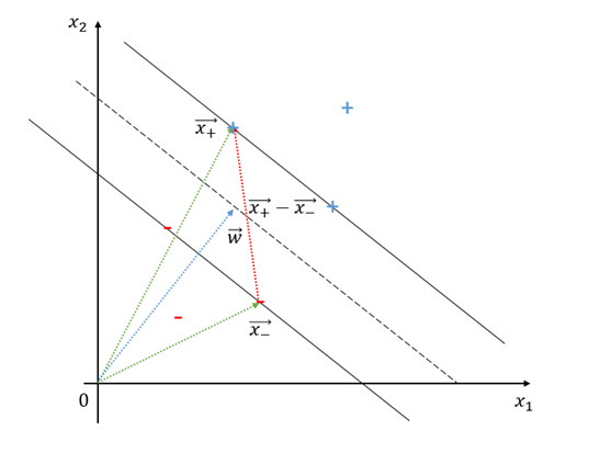
Figure 5. Process for determining the width of the street
Consider the vectors $\vec{x_+}$ and $\vec{x_-}$ from the origin to $x_+$ and $x_-$, respectively, on the solid line in Figure 5. Using $\vec{x_+}-\vec{x_-}$, we can determine the distance between the two solid lines. Since $\vec{w}$ is perpendicular to the dashed line, we can use a unit vector with the same direction as $\vec{w}$ to measure the distance between the two solid lines. The distance between the two solid lines can be expressed as:
\[\frac{\vec{w}}{|\vec{w}|}\cdot(\vec{x}_+ - \vec{x}_-)\]Once again, if $x_i$ was a positive sample, then $y_i=1$ and if $x_i$ was a negative sample, then $y_i=-1$, so:
\[\vec{w}\cdot\vec{x}+b-1 = 0\] \[\Rightarrow \vec{w}\cdot\vec{x}_i = 1-b\]and
\[\vec{w}\cdot\vec{x}+b+1 = 0\] \[\Rightarrow \vec{w}\cdot\vec{x}_i = -1-b\]If we substitute these equations into equation (18), we can determine the distance between the two solid lines.
\[Equation(18) \Rightarrow \frac{1}{|\vec{w}|}(\vec{w}\cdot\vec{x}_+ - \vec{w}\cdot\vec{x}_-)\] \[=\frac{1}{|\vec{w}|}(1-b+1+b)\]\(=\frac{2}{|w|}\) In other words, the distance between two solid lines is $\frac{2}{|\vec{w}|}$, and our goal can be defined as maximizing $\frac{2}{|\vec{w}|}$. Alternatively, we can remove the constant and express it as $max\frac{1}{|\vec{w}|}$ or $min|\vec{w}|$. For mathematical convenience, we can also express it as:
\[min\frac{1}{2}|\vec{w}|^2\]d. Deriving the Lagrange multiplier and constraints
Therefore, the optimization problem we face is as follows:
\[\text{Constraints: } y_i(\vec{w}\cdot\vec{x}_i+b)-1 = 0\] \[\text{Objective function: } \frac{1}{2}|\vec{w}|^2\]Thus, we can set up the following auxiliary equation:
\[L = \frac{1}{2}|\vec{w}|^2 -\sum_i \alpha_i\left[y_i(\vec{w}\cdot \vec{x}_i +b) -1\right]\]Now let’s take partial derivatives of the auxiliary equation with respect to the variables:
\[\frac{\partial L}{\partial \vec{w}} = \vec{w}-\sum_i \alpha_i y_i x_i = 0\] \[\vec{w} = \sum_i \alpha_i y_i \vec{x}_i\]Therefore, $\vec{w}$ is a linear combination of some $\vec{x_i}$’s. We use the term “some” because when $\alpha_i$ is 0, it may not be included in the sum. This means that the algorithm is designed to set the value of $\alpha$ to 0 for samples that do not help set the solid lines, as seen in Figure 4.
Now, if we consider Eq. (31) for the initial boundary decision, we obtain the following constraints:
\[\sum_i \alpha_i y_i \vec{x}_i\cdot\vec{u}+b = +1\text{ for positive class}\] \[\sum_i \alpha_i y_i \vec{x}_i\cdot\vec{u}+b = -1\text{ for negative class}\](Here, once again, only the values of $\pm 1$ appear on the right-hand side because the alpha values for the points that are not on the solid line all become 0.)
Another partial derivative of equation (29) is as follows:
\[\frac{\partial L}{\partial b}=-\sum_i\alpha_i y_i = 0\] \[\Rightarrow \sum_i \alpha_iy_i = 0\]Since the partial derivative with respect to $\alpha_i$ is always 0, we need to use a different method to find the value of $\alpha_i$.
To find $\alpha_i$, we can set up equations (32), (33), and (35) and solve them simultaneously. But let’s go a little further. Let’s substitute equations (31) and (35) into the auxiliary equation $L$ of equation (29).
\[L = \frac{1}{2}|\vec{w}|^2 - \sum_i \alpha_i\left[y_i(\vec{w}\cdot\vec{x}+b)-1\right]\] \[=\frac{1}{2}\left(\sum_i \alpha_i y_i \vec{x}_i\right)\left(\sum_j \alpha_j y_j \vec{x}_j\right) - \sum_i\left(\alpha_iy_i\vec{w}\cdot\vec{x}_i + \alpha_i y_i b - \alpha_i\right)\] \[=\frac{1}{2}\left(\sum_i \alpha_i y_i \vec{x}_i\right)\left(\sum_j \alpha_j y_j \vec{x}_j\right) - \sum_i\left(\alpha_iy_i\vec{x}_i\left(\sum_j\alpha_jy_j\vec{x}_j\right) + \alpha_i y_i b - \alpha_i\right)\] \[=\frac{1}{2}\left(\sum_i \alpha_i y_i \vec{x}_i\right)\left(\sum_j \alpha_j y_j \vec{x}_j\right)-\left(\sum_i \alpha_i y_i\vec{x}_i\right)\left(\sum_j \alpha_j y_j\vec{x}_j\right)-\sum_i\alpha_i y_i b + \sum_i \alpha_i\] \[=\sum_i\alpha_i - \frac{1}{2}\left(\sum_i \alpha_i y_i \vec{x}_i\right)\left(\sum_j \alpha_j y_j \vec{x}_j\right)\] \[=\sum_i\alpha_i - \frac{1}{2}\sum_i\sum_j\alpha_i\alpha_j y_i y_j\vec{x}_i\cdot\vec{x}_j\]e. Kernel Tricks
Looking at equation (41), we can see that the maximum value of L is determined by $\vec{x_i}\cdot\vec{x_j}$. Therefore, if we can appropriately transform $\vec{x_i}\cdot\vec{x_j}$, we can increase the maximum value of $L$.
There are two ways to do this. One is to take an appropriate transformation for $\vec{x_i}$ and $\vec{x_j}$, or to find a transformation $K(\vec{x_i},\vec{x_j})$ that can be substituted for $\vec{x_i}\cdot\vec{x_j}$.
In other words, we can find an appropriate transformation $\phi(\cdot)$ for $\vec{x_i}$, and substitute $\phi(\vec{x_i})\cdot\phi(\vec{x_j})$ instead of $\vec{x_i}\cdot\vec{x_j}$.
Geometrically, this can be easily explained with the following diagram:
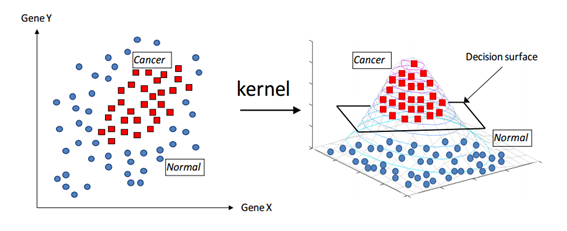
Figure 6. Geometric interpretation of the kernel function. Source: Support Vector Machines without Tears
In Figure 6, the samples on the left plane are transformed to the samples on the right plane, which is done by using the kernel function to transform the sample space into a 3D space. Then, by using a hyperplane in the 3D space, cancer and normal samples can be more easily distinguished.
4. Example of Support Vector Machine Problem
Find the values of $\alpha, b,$ and $w$ for the following + and - samples:
-ve points : A(0,0), B(1,1) +ve points : C(2,0)
Solution)
The positions of the + and - samples are as follows:
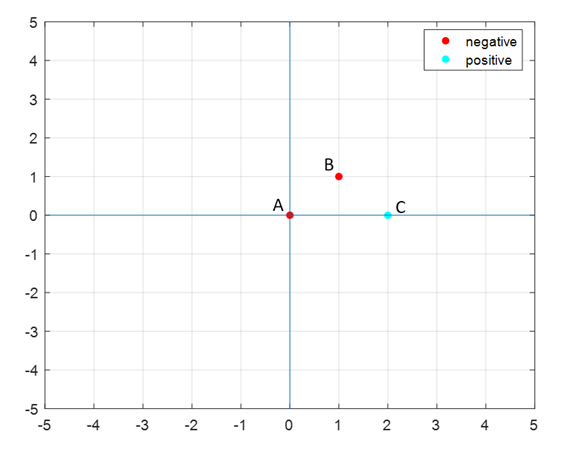
Therefore, at a glance, the equation of the hyperplane seems to be around $y=x-1$. Let’s verify this algebraically.
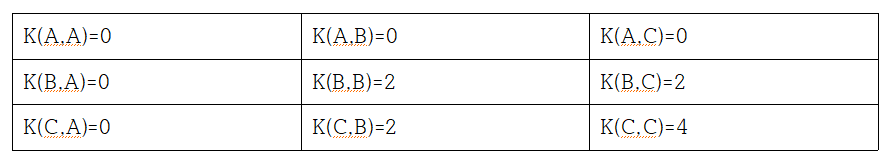
- Step 1) Calculate all kernel function values
In this case, there is nothing special about the kernel function and it is a linear kernel. Therefore,
\[K(\vec{x_1}, \vec{x_2}) = \vec{x}_1\cdot\vec{x}_2\]For all possible cases, we can construct the following table:
- Step 2) Write out the system of equations
From the theory, we can have a total of three constraints:
\[\text{Constraint 1: }\sum_i\alpha_i y_i = 0\] \[\text{Constraint 2: }\sum_i\alpha_i y_i K(x_i, x) + b = 1 \text{ for positive class}\] \[\text{Constraint 3: }\sum_i\alpha_i y_i K(x_i, x) + b = -1 \text{ for negative class}\]Therefore, we can write out the equations using all constraints as follows:
\[C_1: -\alpha_A - \alpha_B + \alpha_C = 0\] \[C_{3, A}: \alpha_A(-1)K(x_A, x_A) + \alpha_B(-1)K(x_B, x_A) + \alpha_C(+1)K(x_C, x_A) + b = -1\] \[C_{3, B}: \alpha_A(-1)K(x_A, x_B) + \alpha_B(-1)K(x_B, x_B) + \alpha_C(+1)K(x_C, x_B) + b = -1\] \[C_{2, C}: \alpha_A(-1)K(x_A, x_C) + \alpha_B(-1)K(x_B, x_C) + \alpha_C(+1)K(x_C, x_C) + b = 1\]After obtaining the values of K in step 1 and substituting them into the four equations above, we can confirm that
\[\alpha_A = 0, \alpha_B = 1, \alpha_C = 1, b = -1\]Therefore, we can also see that point A is not a support vector.
And $\vec{w}$ can be calculated as
\[\vec{w} = \sum_i\alpha_i y_i\vec{x}_i\] \[=\alpha_A y_i \vec{x}_A + \alpha_B y_i \vec{x}_B + \alpha_C y_i \vec{x}_C\] \[= 0 + (1)(-1)\begin{bmatrix}1 \\1 \end{bmatrix} + (1)(1)\begin{bmatrix}2 \\0\end{bmatrix}\] \[=\begin{bmatrix}1 \\ -1\end{bmatrix}\]Therefore, the equation for the hyperplane is
\[\vec{w}\cdot\vec{x}+b = 0\]which becomes
\[x_1-x_2 - 1 = 0\]and can be easily expressed as the equation for a straight line:
\(y = x - 1\) The result matches the one obtained using MATLAB’s fitcsvm function. Here is the model obtained using fitcsvm, where beta represents $\vec{w}$ and bias represents b, which we used in the hyperplane equation.
The code used for this example is given below.
clear all; close all; clc;

X=[0 0;1 1;2 0];
Y=['negative';'negative';'positive'];

SVMModel=fitcsvm(X,Y);


sv = SVMModel.SupportVectors;
figure
gscatter(X(:,1),X(:,2),Y)
hold on
plot(sv(:,1),sv(:,2),'ko','MarkerSize',10)
legend('+','-','Support Vector')
grid on;
xlim([-5 5])
ylim([-5 5])
line([-5 5],[0 0])
line([0 0],[-5 5])

w=SVMModel.Beta
b=SVMModel.Bias

% Therefore, the equation is 1*x+(-1)*y-1=0
% which means y=x-1.
x=linspace(-5,5,100);
y=-1*(w(1)/w(2))*x+b;
plot(x,y)